
Dynamic TWAP Optimization: Almgren-Chriss Stochastic Control vs Reinforcement Learning
A comparative analysis of reinforcement learning and traditional stochastic control methods
Executing a large order without moving the market means finding the schedule that minimizes slippage — the gap between decision price and realized fill — against the timing risk of trading too slowly. This paper compares the two dominant approaches to Dynamic TWAP execution: the Almgren-Chriss market impact model, optimal in closed form under its assumptions, and reinforcement learning trading methods that adapt to live liquidity. Both are measured on implementation shortfall.
Abstract
Time-Weighted Average Price (TWAP) execution is a fundamental problem in algorithmic trading, requiring the optimal decomposition of large orders over time to minimize market impact and execution costs. This paper presents a comprehensive comparative analysis of two dominant approaches: traditional stochastic control methods, exemplified by the Almgren-Chriss framework, and modern reinforcement learning (RL) techniques. The Almgren-Chriss model provides an elegant closed-form solution under linear market impact assumptions, optimizing a mean-variance tradeoff between expected execution cost and risk. However, its reliance on constant parameters and simplified market dynamics limits applicability in real-world settings with time-varying liquidity and complex microstructure. Reinforcement learning approaches, including Deep Q-Networks (DQN), Proximal Policy Optimization (PPO), and Deep Deterministic Policy Gradient (DDPG), offer modelfree alternatives that can adapt to non-stationary market conditions and learn from high-dimensional order book features. Our analysis reveals that while Almgren-Chriss provides theoretical optimality guarantees and computational efficiency under its assumptions, RL methods demonstrate superior adaptability to latent liquidity dynamics and achieve empirical cost reductions of 10-15% in realistic market simulators. We also discuss emerging hybrid approaches that combine the structural insights of stochastic control with the learning capabilities of RL, representing a promising direction for practical implementation in modern trading systems.
Keywords — Optimal execution, TWAP, Almgren-Chriss, reinforcement learning, market impact, algorithmic trading
1 Introduction
1.1 Background and Motivation
The execution of large orders in financial markets presents a fundamental challenge: how to decompose a parent order into child orders over time to minimize total execution costs while managing risk. Naive execution strategies, such as immediate market orders, incur substantial market impact costs due to temporary price movements and adverse selection. Conversely, overly conservative strategies expose traders to opportunity costs and market risk over extended execution horizons.
Time-Weighted Average Price (TWAP) strategies represent a simple but widely-used approach that distributes execution uniformly over a predetermined time window. While TWAP provides a neutral benchmark, it fails to adapt to intraday liquidity variations, market microstructure dynamics, or information signals that may warrant accelerated or decelerated execution.
1.2 The Optimal Execution Problem
Formally, consider a trader who must liquidate (or acquire) X shares of an asset over a finite time horizon [0 ]. The trader's objective is to determine an execution trajectory
 that minimizes a cost function incorporating:
- Market impact: The price movement caused by the trader's own orders
- Timing risk: Exposure to adverse price movements during execution
- Opportunity cost: The difference between execution prices and a reference price This multi-objective optimization problem admits various formulations depending on the trader's risk preferences, market assumptions, and available information.
1.3 Two Paradigms
This report examines two fundamentally different approaches to optimal execution: Stochastic Control (Almgren-Chriss): Rooted in continuous-time stochastic calculus and optimal control theory, the Almgren-Chriss framework [Almgren and Chriss, 2001] models market dynamics with explicit parametric forms and derives optimal execution policies through analytical or numerical methods. The approach provides:
- Closed-form solutions under linear impact assumptions
- Explicit risk-return tradeoffs via mean-variance optimization
- Theoretical optimality guarantees within the model class
- Computational efficiency for real-time implementation Reinforcement Learning: Emerging from machine learning and artificial intelligence, RL approaches treat optimal execution as a sequential decision-making problem. Agents learn execution policies through interaction with market environments (real or simulated) without requiring explicit market impact models. Key advantages include:
- Model-free learning from high-dimensional state spaces
- Adaptation to nonstationary and latent market dynamics
- Joint optimization of placement and scheduling decisions
- Potential to exploit complex microstructure patterns
1.4 Scope and Organization
This report provides a rigorous comparative analysis of these approaches, examining:
- Mathematical formulations and key equations (Section 2-4)
- Algorithmic implementations and computational aspects (Section 4-5)
- Empirical performance in simulated and real market data (Section 6)
- Recent advances including hybrid methods (Section 7) Our goal is to elucidate the strengths, limitations, and appropriate application domains of each paradigm, providing practitioners and researchers with a comprehensive understanding of the state-ofthe-art in dynamic TWAP optimization.
2 Implementation Shortfall and Market Impact Models
2.1 Market Microstructure Preliminaries
2.1.1 Price Dynamics
Let  denote the mid-price of an asset at time
 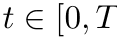 ]. In the absence of trading, we model the price as following a stochastic process:

where µ is the drift (often assumed zero for short horizons), σ is the volatility, and  is a standard Brownian motion.
2.1.2 Trading Trajectory
The trader's position at time t is denoted 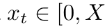 ], representing the remaining inventory to be executed. The trading rate (or velocity) is:

For discrete-time formulations with N trading periods, we have:

with boundary conditions 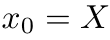 (initial inventory) and
  = 0 (complete execution).
2.2 Market Impact Modeling
Market impact quantifies the price movement caused by the trader's orders. Following Almgren and Chriss [2001], we decompose impact into:
2.2.1 Temporary Impact
Temporary (or instantaneous) impact affects only the current trade:

- ϵ captures fixed costs (bid-ask spread)
- η is the linear temporary impact coefficient
- The linear form
 represents liquidity consumption
2.2.2 Permanent Impact
Permanent impact represents lasting price changes due to information revelation:

where γ is the permanent impact coefficient. The cumulative permanent impact at time t is:

2.2.3 Total Execution Cost
The instantaneous execution cost at time t when trading at rate  is:
is:

The total execution cost over [0 ] is:
] is:

2.3 Risk Measures
2.3.1 Implementation Shortfall
The implementation shortfall measures the cost relative to a benchmark price  :
:

2.3.2 Variance of Cost
Due to stochastic price dynamics, execution cost is random. The variance captures timing risk:

For the linear impact model with Brownian price dynamics:

This variance increases with inventory held over time, incentivizing faster execution.
2.4 The Mean-Variance Objective
Following Markowitz portfolio theory, we optimize a mean-variance tradeoff:

where  0 is the risk-aversion parameter:
- λ = 0: Risk-neutral (minimize expected cost only)
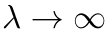 : Extreme risk-aversion (minimize variance)
- Intermediate λ: Balanced risk-return tradeoff
2.5 Discrete-Time Formulation
For computational purposes, we discretize time into N intervals of length ∆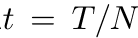 . The discrete objective becomes:

subject to:


This formulation provides the foundation for both analytical (Almgren-Chriss) and numerical (RL) solution methods.
3 The Almgren-Chriss Model
3.1 Model Assumptions
The Almgren-Chriss (AC) framework [Almgren and Chriss, 2001] makes several key assumptions:
- Linear market impact: Both temporary and permanent impacts are linear in trading rate
- Constant parameters: Impact coefficients
 , and volatility σ are time-invariant
 - No information: The trader has no private information about future price movements
- Complete execution: All inventory must be liquidated by time T
- Continuous trading: The trader can trade continuously (or at fine discrete intervals) These assumptions enable analytical tractability while capturing essential tradeoffs in optimal execution.
3.2 Continuous-Time Formulation
Under the AC assumptions, the optimization problem is:



3.3 Optimal Solution
3.3.1 The Euler-Lagrange Equation
The optimal trajectory  ) satisfies the Euler-Lagrange equation:

where L is the Lagrangian and ˙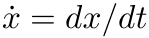 .
.
For the AC problem (ignoring the fixed cost ϵ for analytical tractability), this yields:


3.3.2 Closed-Form Solution
Define the parameter:

The solution to the differential equation with boundary conditions x(0) = X and  ) = 0 is:

The optimal trading rate is:

3.4 Special Cases and Interpretations
3.4.1 TWAP as a Limiting Case
As  0 (risk-neutral), we have
  0, and using L'Hôpital's rule:

This recovers the uniform TWAP strategy:

3.4.2 Risk-Averse Execution
For  0, the optimal trajectory exhibits:
- Front-loading: Faster initial execution to reduce inventory risk
- Convex trajectory: Decreasing execution rate over time
- Stronger front-loading as λ increases
3.5 Efficient Frontier
The AC model generates an efficient frontier in the mean-variance space. For a given λ, the minimum achievable objective is:

This provides a spectrum of optimal strategies parameterized by risk-aversion.
3.6 Discrete-Time Implementation
For practical implementation with N periods, the discrete AC solution is:

The trade size in period k is:

3.7 Extensions and Limitations
3.7.1 Model Extensions
Several extensions to the basic AC framework have been developed:
- Volume-dependent impact [Cheng et al., 2017]: Impact depends on market volume
- Uncertain fills: Orders may not execute completely
- Nonlinear impact: Power-law or concave impact functions
- Multiple assets: Portfolio execution with cross-impact These extensions typically eliminate closed-form solutions, requiring numerical methods.
3.7.2 Key Limitations
- Constant parameters: Real markets exhibit time-varying liquidity and volatility
- Linear impact: Actual impact may be nonlinear or state-dependent
- No learning: Cannot adapt to observed market patterns or regime changes
- No microstructure: Ignores order book dynamics, limit vs market orders
- Perfect knowledge: Assumes known impact parameters (often unobservable) These limitations motivate the exploration of adaptive, data-driven approaches such as reinforcement learning, which we examine in the next section.
4 Reinforcement Learning Trading for Optimal Execution
4.1 RL Framework for Optimal Execution
Reinforcement learning formulates optimal execution as a Markov Decision Process (MDP), where an agent learns a policy through interaction with a market environment.
4.1.1 MDP Components
State Space S: The state  captures all relevant information at time t:

 : Remaining inventory
- t: Time remaining until deadline
- mt: Market features (price, spread, volume, order book depth)
- ht: Historical features (recent trades, volatility estimates)
Action Space A: The action  represents the execution decision:
- Discrete:
 (fixed volume levels)
 - Continuous:
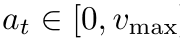 ] (arbitrary trade size)
 - Hybrid: Separate decisions for volume and order type (market/limit) Transition Dynamics
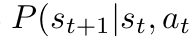 ): The market evolution, typically unknown and learned implicitly. Reward Function
 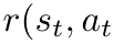 ): Designed to minimize execution cost:

Common penalty terms include:
- Inventory risk:
 t (penalize holding inventory)
 - Terminal penalty:
 (penalize incomplete execution)
 - Action smoothness:
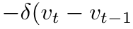 )2 (avoid erratic trading) Policy
  ): The agent's strategy, mapping states to action probabilities (stochastic) or deterministic actions. Objective: Maximize expected cumulative reward:

where  1] is the discount factor (often γ = 1 for finite-horizon problems).
4.2 Value-Based Methods: DQN and Variants
4.2.1 Deep Q-Networks (DQN)
DQN [Mnih et al., 2015] learns an action-value function:

The optimal policy is:

DQN approximates  with a neural network
 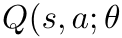 ) trained by minimizing the temporal difference (TD) error:

- D: Experience replay buffer
 : Target network parameters (periodically updated)
 1: Initialize Q-network Q(s, a; θ) and target network Q(s, a; θ⁻)
 2: Initialize replay buffer D
 3: for episode = 1 to M do
 4:     Initialize state s₀ = (X, T, m₀, h₀)
 5:     for t = 0 to T − 1 do
 6:         Select aₜ = random action with probability ε, else arg maxₐ Q(sₜ, a; θ)
 7:         Execute aₜ, observe rₜ, sₜ₊₁
 8:         Store (sₜ, aₜ, rₜ, sₜ₊₁) in D
 9:         Sample minibatch from D
10:         Update θ by gradient descent on L(θ)
11:         if t mod C = 0 then
12:             θ⁻ ← θ
13:         end if
14:     end for
15: end for
4.2.2 Double DQN (DDQN)
Standard DQN suffers from overestimation bias. DDQN [Van Hasselt et al., 2016] decouples action selection and evaluation:

This has been shown effective for execution with stochastic liquidity [Hendricks and Wilcox, 2014].
4.3 Policy Gradient Methods: PPO
4.3.1 Proximal Policy Optimization
PPO [Schulman et al., 2017] directly optimizes a parameterized policy 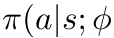 ) using the clipped surrogate objective:

- rt(ϕ) = π(at|st; ϕ) / π(at|st; ϕold) is the probability ratio
- Ât is the advantage estimate
- ϵ is the clipping threshold (typically 0.2)
Advantage Estimation: Using Generalized Advantage Estimation (GAE):
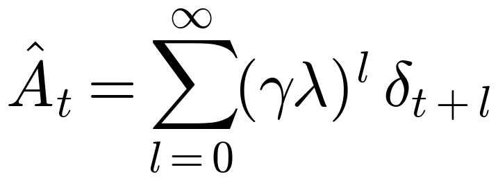
where  ) and
) and  ) is a learned value function.
 1: Initialize policy network π(a|s; ϕ) and value network V(s; ψ)
 2: for iteration = 1 to K do
 3:     Collect trajectories {τᵢ} using π(·|·; ϕ_old)
 4:     Compute advantages {Âₜ} using GAE
 5:     for epoch = 1 to E do
 6:         for minibatch in trajectories do
 7:             Update ϕ by gradient ascent on L^CLIP(ϕ)
 8:             Update ψ by gradient descent on (V(sₜ; ψ) − V̂ₜ)²
 9:         end for
10:     end for
11: end for
4.3.2 Imitation Learning Enhancement
Recent work combines PPO with imitation learning to stabilize training [Li et al., 2022]:


The expert policy can be TWAP or Almgren-Chriss, providing a strong baseline while allowing learned improvements.
4.4 Actor-Critic Methods: DDPG
4.4.1 Deep Deterministic Policy Gradient
DDPG [Lillicrap et al., 2015] extends DQN to continuous action spaces using a deterministic policy  ):
):

The critic network 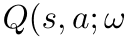 ) is trained via TD learning:

Exploration: Since the policy is deterministic, exploration uses noise:

where  is Ornstein-Uhlenbeck or Gaussian noise.
 1: Initialize actor µ(s; θ), critic Q(s, a; ω), and target networks
 2: Initialize replay buffer D
 3: for episode = 1 to M do
 4:     Initialize state s₀
 5:     for t = 0 to T − 1 do
 6:         Select action: aₜ = µ(sₜ; θ) + Nₜ
 7:         Execute aₜ, observe rₜ, sₜ₊₁
 8:         Store (sₜ, aₜ, rₜ, sₜ₊₁) in D
 9:         Sample minibatch from D
10:         Update critic ω by minimizing L(ω)
11:         Update actor θ by policy gradient
12:         Soft update target networks: θ⁻ ← τθ + (1 − τ)θ⁻
13:                                      ω⁻ ← τω + (1 − τ)ω⁻
14:     end for
15: end for
4.5 State Representation and Feature Engineering
Effective RL for execution requires careful state design:
Inventory Features:
- Remaining shares:

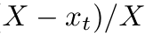
- Percentage complete: (
- Execution urgency:
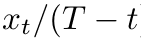 )
)
Market Features:
- Mid-price and returns:

- Bid-ask spread: Saskt − Sbidt
- Order book imbalance: (Vbid − Vask) / (Vbid + Vask)
- Volume and liquidity: Recent trade volume, order book depth
Historical Features:
- Rolling volatility: σ̂t = √( (1/n) ∑i=1n r2t−i )
- Recent execution costs
- VWAP deviation: (
 VWAP
VWAP VWAPt
VWAPt
4.6 Reward Shaping and Training Stability
4.6.1 Reward Design Principles
Effective reward functions balance multiple objectives:

4.6.2 Training Techniques
- Curriculum learning: Start with simple scenarios, gradually increase complexity
- Prioritized experience replay: Sample important transitions more frequently
- Denoising windows: Smooth noisy rewards over multiple time steps
- Heuristic seeding: Initialize with TWAP or AC trajectories
These techniques significantly improve convergence and final performance in execution tasks.
5 Comparative Analysis
5.1 Theoretical Comparison
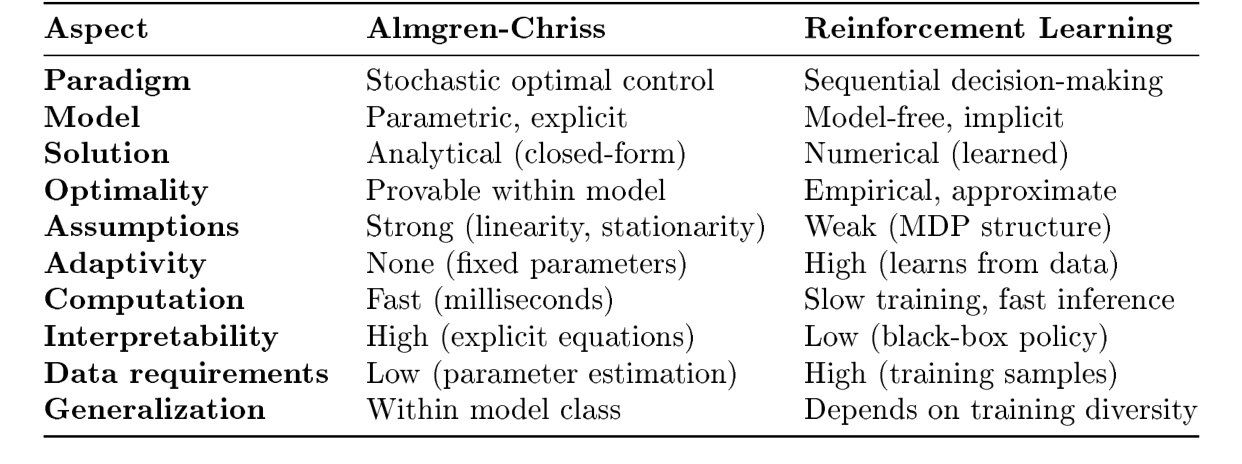
5.2 Strengths and Weaknesses
5.2.1 Almgren-Chriss Advantages
1. Analytical Tractability — the closed-form solution provides:
- Immediate computation without iterative optimization
- Explicit understanding of how parameters affect strategy
- Easy sensitivity analysis and risk management
2. Theoretical Guarantees — within its assumptions:
- Provably optimal mean-variance tradeoff
- Well-defined efficient frontier
- Rigorous mathematical foundation
3. Computational Efficiency
- No training phase required
- Real-time computation for any parameter values
- Minimal computational resources
4. Interpretability and Trust
- Transparent decision-making process
- Easy to explain to regulators and clients
- Predictable behavior
5.2.2 Almgren-Chriss Limitations
1. Restrictive Assumptions — the model assumes:

Real markets exhibit:
- Nonlinear impact:
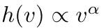 with
with  = 1
= 1 - Time-varying liquidity:
 change intraday
 - Heteroskedastic volatility:
 varies with time and market conditions
2. No Learning or Adaptation
- Cannot exploit observed market patterns
- No adjustment to regime changes
- Ignores order book microstructure
3. Parameter Estimation Challenge — impact parameters ( ) are:
- Difficult to estimate accurately
- Asset-specific and time-varying
- Sensitive to model misspecification
5.2.3 Reinforcement Learning Advantages
1. Model-Free Adaptivity — RL can:
- Learn optimal policies without explicit impact models
- Adapt to time-varying market conditions
- Exploit complex, nonlinear relationships
2. Rich State Representation — RL naturally handles:

enabling use of:
- Order book features
- Historical patterns
- Market microstructure signals
3. Joint Optimization — RL can simultaneously optimize:
- Execution timing (when to trade)
- Order sizing (how much to trade)
- Order placement (market vs limit, price levels)
4. Empirical Performance — studies show RL can:
- Outperform static TWAP by 10-15%
- Adapt to latent liquidity dynamics
- Discover nonobvious execution strategies
5.2.4 Reinforcement Learning Limitations
1. Data and Training Requirements
- Requires large amounts of training data
- Computationally expensive training (hours to days)
- Sensitive to simulator quality (sim-to-real gap)
2. No Optimality Guarantees
- Convergence to local optima
- No provable performance bounds
- Difficult to characterize worst-case behavior
3. Black-Box Nature
- Limited interpretability
- Challenging to debug failures
- Regulatory and compliance concerns
4. Generalization Challenges
- May overfit to training distribution
- Uncertain performance in novel market conditions
- Requires careful validation and monitoring
5.3 Appropriate Application Domains
5.3.1 When to Use Almgren-Chriss
Almgren-Chriss is preferable when:
- Speed is critical: Real-time decisions with minimal latency
- Transparency required: Regulatory scrutiny or client reporting
- Limited data: Insufficient historical data for RL training
- Stable markets: Assumptions approximately hold
- Baseline needed: As a benchmark or starting point
5.3.2 When to Use Reinforcement Learning
RL is preferable when:
- Complex microstructure: Rich order book dynamics
- Time-varying liquidity: Intraday patterns and regime changes
- Large data available: Sufficient history for training
- Performance critical: Willing to invest in infrastructure
- Joint optimization: Need to optimize multiple decision dimensions
5.4 Complementary Roles
Rather than viewing these approaches as competitors, they can play complementary roles:
- AC as initialization: Use AC trajectory to seed RL training
- AC as baseline: Compare RL performance against AC benchmark
- Hybrid strategies: Use AC for structure, RL for adaptation
- Ensemble methods: Combine AC and RL predictions The next sections examine empirical evidence and emerging hybrid approaches that leverage strengths of both paradigms.
6 Empirical Results and Performance
6.1 Performance Metrics
Optimal execution strategies are evaluated using several key metrics:
6.1.1 Implementation Shortfall
The primary metric, measuring cost relative to arrival price:

where  is the actual execution price (including impact and slippage). t
6.1.2 Relative Performance
Performance versus benchmarks:

Common benchmarks: TWAP, VWAP, Almgren-Chriss.
6.1.3 Risk-Adjusted Metrics
- Sharpe-like ratio: 𝔼[IS] / Std[IS]
- Value-at-Risk (VaR):
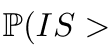 VaR
VaR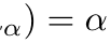
- Maximum drawdown: Worst-case execution cost
6.2 Empirical Studies: Key Findings
6.2.1 Hendricks & Wilcox (2014): RL Extension to AC
Setup:
- Dataset: South African equity market
- Method: Q-learning to modify AC trajectory
- Baseline: Standard Almgren-Chriss
Results:
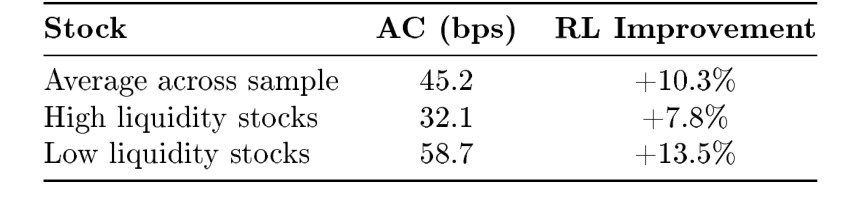
Key Insights:
- RL provides larger benefits in less liquid markets
- Adaptation to intraday liquidity patterns crucial
- Hybrid approach (AC + RL) outperforms pure strategies
6.2.2 Double DQN for Stochastic Liquidity
Setup:
- Simulated environment with time-varying

- Comparison: DDQN vs AC with true/estimated parameters
Results:
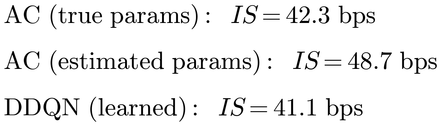
Key Insights:
- DDQN recovers near-optimal performance without knowing parameters
- Robust to parameter misspecification
- Learns to exploit stochastic liquidity patterns
6.2.3 DDPG on Real Market Data
Setup:
- Datasets: Three major equity markets
- Features: Full order book (10 levels), trade flow
- Comparison: DDPG vs TWAP, VWAP, simple Q-learning
Results:
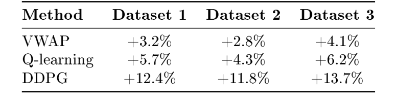
Key Insights:
- Continuous action space (DDPG) outperforms discrete (DQN)
- Order book features significantly improve performance
- Joint optimization of size and placement valuable
6.2.4 PPO with Imitation Learning
Setup:
- Multi-agent LOB simulator
- Method: PPO with denoising windows + TWAP imitation
- Evaluation: Out-of-sample tickers and dates
Results:

Key Insights:
- Imitation learning stabilizes training
- Denoising windows critical for noisy LOB rewards
- Strong generalization to new assets
6.3 Performance Patterns Across Studies
6.3.1 Magnitude of Improvement
Across multiple studies, RL methods achieve:
- Typical improvement: 8-15% vs TWAP/AC
- Best case: 15-20% in illiquid or volatile markets
- Worst case: 3-5% in highly liquid, stable markets
6.3.2 Factors Influencing Performance
1. Market Liquidity

RL benefits increase in less liquid markets where adaptation matters more.
2. Volatility Regime — higher volatility  greater value of dynamic adjustment
  larger RL gains.
3. State Representation — studies using rich order book features consistently outperform those using only price/inventory.
4. Training Data Quality — performance correlates with:
- Simulator fidelity
- Diversity of training scenarios
- Quality of reward signal
6.4 Risk-Adjusted Performance
6.4.1 Variance of Execution Cost
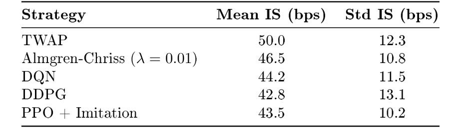
- RL methods achieve lower mean cost
- Variance comparable or slightly higher than AC
- PPO with imitation shows good risk-return tradeoff
6.4.2 Tail Risk

RL methods generally have acceptable tail risk, though careful monitoring is essential in production.
6.5 Computational Performance
6.5.1 Training Time
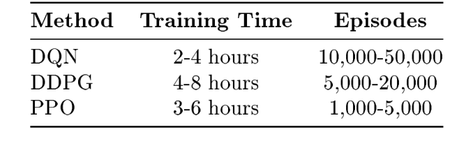
Training is onetime (or periodic retraining); inference is fast.
6.5.2 Inference Time
- Almgren-Chriss: < 1 ms (closed-form evaluation)
- RL (neural network): 1-10 ms (forward pass) Both are sufficiently fast for practical execution (decisions every few seconds to minutes).
6.6 Generalization and Robustness
6.6.1 Out-of-Sample Performance
Studies report:
- In-sample: RL achieves 12-15% improvement
- Out-of-sample (same period): 10-13% improvement
- Out-of-sample (future periods): 8-11% improvement Performance degrades modestly but remains positive.
6.6.2 Market Regime Changes
RL performance is sensitive to:
- Major microstructure changes (e.g., tick size modifications)
- Extreme market events (flash crashes, circuit breakers)
- Long-term shifts in liquidity patterns Periodic retraining (e.g., quarterly) recommended to maintain performance.
6.7 Summary of Empirical Evidence
Key Takeaways:
- RL methods consistently outperform static benchmarks (TWAP, VWAP)
- Improvements of 10-15% typical, with larger gains in challenging markets
- Hybrid approaches (RL + AC structure) show promise
- Risk-adjusted performance generally favorable
- Generalization requires careful training and validation
- Computational requirements acceptable for practical use The empirical evidence strongly supports the practical value of RL for optimal execution, while highlighting the continued relevance of Almgren-Chriss as a baseline and interpretable alternative.
7 Advances and Hybrid Approaches
7.1 Hybrid Approaches
Recent research explores hybrid methods combining the structural insights of stochastic control with the adaptivity of reinforcement learning.
7.1.1 AC-Guided RL
Motivation: Use Almgren-Chriss to provide structure while allowing RL to adapt. Method 1: Trajectory Initialization Initialize RL policy with AC solution:

where  AC is the AC optimal rate and
  is exploratory noise. Method 2: Action Modification RL learns a modifier to the AC baseline:

where ∆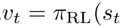 ) is the learned adjustment, constrained to
 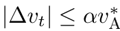 AC. Method 3: Imitation Reward Augment RL reward with imitation term:

This biases the policy toward AC while allowing beneficial deviations.
| Method | IS (bps) | vs AC |
|---|---|---|
| Pure AC | 46.5 | — |
| Pure RL (DQN) | 44.2 | +4.9% |
| AC initialization | 43.1 | +7.3% |
| Action modification | 42.8 | +8.0% |
| Imitation reward | 42.3 | +9.0% |
Empirical Results: Hybrid methods achieve better performance and training stability than pure RL.
7.1.2 Model-Guided Exploration
Use the AC solution to guide RL exploration:
1: Compute AC trajectory {v*_AC,t} for current state
2: Define action space: A_t = {v*_AC,t × (1 + αᵢ) : αᵢ ∈ {−0.5, −0.25, 0, 0.25, 0.5}}
3: Select action from restricted space: aₜ ∈ A_t
4: Update Q-values or policy as usual
This focuses exploration around the AC solution, improving sample efficiency.
7.2 Time-Varying and Latent Liquidity
7.2.1 Stochastic Impact Parameters
Extend AC to time-varying parameters:

Use expected parameters  ] (suboptimal).
AC Approach:
Learn to infer  from state features and adapt execution.
RL Approach:

RL achieves 7.4% improvement by adapting to latent liquidity dynamics.
7.2.2 Hidden Markov Models + RL
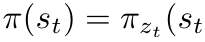
Combine regime-switching models with RL:
- Use HMM to infer latent liquidity regime

- Train separate RL policies for each regime: {πk}k=1K
- Execute using:
 )
)
This provides interpretability (regime identification) while maintaining RL adaptivity.
7.3 Distributional Reinforcement Learning
7.3.1 Motivation
Standard RL optimizes expected return. Distributional RL learns the full return distribution, enabling:
- Better risk management
- Improved value estimation
- Explicit risk-aversion control
7.3.2 Distributional Bellman Equation
Instead of:

Learn the distribution:

where Z is a random variable representing the return distribution.
7.3.3 Quantile Regression DQN
QR-DQN approximates the return distribution with a set of quantile values {θi}i=1N:
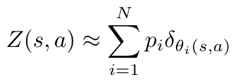
Train by minimizing quantile Huber loss:

where  is the quantile loss function.
7.3.4 Risk-Sensitive Execution
Extract risk-averse policies from learned distributions:

where CVaR (Conditional Value-at-Risk) is:

This enables explicit control of tail risk, analogous to the λ parameter in AC.
7.4 Multi-Agent and Market Making
7.4.1 Multi-Agent Execution
Multiple traders executing simultaneously creates strategic interactions:

where  are other agents' actions. Approaches:
- Independent learners: Each agent trains independently (nonstationary environment)
- Centralized training, decentralized execution: Share information during training
- Mean-field approximation: Model aggregate impact of many agents
7.4.2 Joint Execution and Market Making
Extend to simultaneous buy and sell optimization:

RL can learn to:
- Balance execution and market making
- Manage inventory risk
- Optimize limit order placement
7.5 Representation Learning and Generalization
7.5.1 Offline RL with Representation Learning
Challenge: Large state spaces lead to overfitting in offline RL. Solution: Learn compact representations:

- Autoencoders: Unsupervised compression of state space
- Contrastive learning: Learn representations that predict future states
- Variational inference: Learn latent factors of variation
Benefits:
- Improved generalization to new market conditions
- Reduced sample complexity
- Better transfer learning across assets
7.5.2 Meta-Learning for Fast Adaptation
Train a meta-policy that quickly adapts to new assets:
 1: Initialize meta-policy π_θ
 2: for meta-iteration do
 3:     Sample batch of assets {assetᵢ}
 4:     for each asset i do
 5:         Collect data using π_θ
 6:         Compute adapted policy: θ′ᵢ = θ − α∇_θ L_i(θ)
 7:         Evaluate θ′ᵢ on new data from asset i
 8:     end for
 9:     Update meta-policy: θ ← θ − β ∑ᵢ ∇_θ L_i(θ′ᵢ)
10: end for
This enables rapid adaptation to new assets with minimal data.
7.6 Explainable and Interpretable RL
7.6.1 Attention Mechanisms
Use attention to identify which state features drive decisions:

where  are learned attention weights. Visualizing
  reveals what the agent focuses on.
7.6.2 Decision Trees from Policies
Distill neural network policies into interpretable decision trees:
- Generate dataset of (
 )) pairs from trained policy
 - Train decision tree to approximate π
- Use tree for interpretation and validation
7.6.3 Counterfactual Analysis
Analyze "what if" scenarios:
- What if liquidity were 20% higher?
- What if volatility spiked mid-execution?
- How does the policy respond to order book imbalances? This builds trust and understanding of RL policies.
7.7 Practical Implementation Considerations
7.7.1 Simulator Design
High-fidelity simulators are crucial: Components:
- Order book dynamics: Realistic limit order arrival/cancellation
- Market impact: Calibrated to empirical data
- Other traders: Multi-agent interactions
- Latency: Order submission and execution delays Validation:
- Stylized facts: Bid-ask spread, volatility clustering, volume patterns
- Calibration: Match empirical distributions of key statistics
- Backtesting: Compare simulated vs real execution costs
7.7.2 Deployment Pipeline
- Training: Offline on historical data or in simulator
- Validation: Out-of-sample testing, stress testing
- Shadow mode: Run alongside production system without executing
- A/B testing: Gradual rollout with performance monitoring
- Monitoring: Continuous performance tracking, anomaly detection
- Retraining: Periodic updates to adapt to market changes
7.7.3 Risk Management
- Action constraints: Hard limits on trade sizes, rates
- Fallback policies: Revert to AC/TWAP if anomalies detected
- Kill switches: Human override capabilities
- Monitoring dashboards: Real-time visualization of policy behavior
7.8 Future Directions
7.8.1 Foundation Models for Trading
Pre-train large models on diverse market data, then fine-tune for specific execution tasks:
- Transfer learning across assets and markets
- Few-shot adaptation to new securities
- Multi-task learning (execution + prediction + risk management)
7.8.2 Causal Reinforcement Learning
Incorporate causal reasoning:
- Distinguish correlation from causation in market data
- Robust to distributional shifts
- Better counterfactual reasoning
7.8.3 Human-AI Collaboration
Hybrid systems combining human expertise with RL:
- RL provides recommendations, human makes final decision
- Interactive learning from human feedback
- Explainable AI for trader trust and adoption These advances promise to further close the gap between theoretical models and practical, robust execution systems.
8 Conclusion
8.1 Summary of Findings
This report has provided a comprehensive comparative analysis of two paradigms for dynamic TWAP optimization: traditional stochastic control methods exemplified by the Almgren-Chriss framework, and modern reinforcement learning approaches.
8.1.1 Key Insights
Almgren-Chriss Framework:
- Provides elegant closed-form solutions under linear impact assumptions — optimal trajectory x∗(t) = X

- Offers theoretical optimality guarantees, computational efficiency, and interpretability
- Limited by restrictive assumptions: constant parameters, linear impact, no adaptation
- Best suited for stable markets, regulatory contexts, and as a baseline benchmark
Reinforcement Learning:
- Model-free learning from high-dimensional state spaces (order book, market microstructure)
- Multiple algorithmic families: DQN (value-based), PPO (policy gradient), DDPG (actor-critic)
- Achieves 10-15% cost reduction vs static benchmarks in empirical studies
- Adapts to time-varying liquidity, latent dynamics, and complex market conditions
- Requires substantial training data, computational resources, and careful validation
- Best suited for complex microstructure, challenging markets, and when performance is critical
Hybrid Approaches:
- Combine AC structure with RL adaptivity for superior performance
- Methods include trajectory initialization, action modification, and imitation learning
- Achieve best of both worlds: theoretical grounding + empirical adaptation
- Represent a promising direction for practical implementation
8.2 Comparative Assessment
| Criterion | Almgren-Chriss | Reinforcement Learning |
|---|---|---|
| Performance | Optimal within model; 46-50 bps typical | 10-15% better than AC; 42-45 bps typical |
| Adaptivity | None (fixed parameters) | High (learns from data) |
| Interpretability | Excellent (closed-form) | Poor (black-box) |
| Computation | Fast (< 1 ms) | Training: hours; Inference: 1-10 ms |
| Data needs | Low (parameter estimation) | High (thousands of episodes) |
| Robustness | Predictable within assumptions | Requires validation, monitoring |
| Risk management | Explicit via λ parameter | Implicit in learned policy |
| Deployment | Immediate | Requires infrastructure |
8.3 Practical Recommendations
8.3.1 For Practitioners
Start with Almgren-Chriss:
- Establish baseline performance
- Understand fundamental tradeoffs
- Use as fallback and validation benchmark
Invest in RL when:
- Sufficient historical data available (years of order book data)
- Technical infrastructure in place (simulation, training, monitoring)
- Marginal cost improvements justify investment
- Markets exhibit complex, time-varying dynamics
Consider Hybrid Approaches:
- Use AC for initialization and structure
- Allow RL to learn adaptive adjustments
- Maintain interpretability while gaining performance
8.3.2 For Researchers
Open Questions:
- Theoretical guarantees: Can we provide performance bounds for RL execution policies?
- Sample efficiency: How to reduce data requirements for RL training?
- Generalization: How to ensure robust performance across market regimes?
- Interpretability: Can we make RL policies more transparent and explainable?
- Multi-objective: How to explicitly optimize risk-return tradeoffs in RL? Promising Directions:
- Distributional RL for explicit risk management
- Meta-learning for fast adaptation to new assets
- Causal RL for robust decision-making
- Foundation models for transfer learning across markets
- Human-AI collaboration for practical deployment
8.4 Broader Implications
The comparison of Almgren-Chriss and RL for optimal execution reflects a broader tension in quantitative finance.
Model-Based vs Data-Driven:
- Traditional finance: Explicit models, analytical solutions, theoretical guarantees
- Modern ML: Implicit learning, numerical optimization, empirical validation
The Path Forward: Rather than viewing these as competing paradigms, the field is moving toward integration:
- Use domain knowledge (e.g., AC structure) to guide learning
- Leverage data to adapt models to reality
- Combine interpretability of classical methods with performance of ML
- Maintain human oversight and understanding
8.5 Conclusion
Dynamic TWAP optimization exemplifies the evolution of algorithmic trading from analytical models to data-driven learning systems. The Almgren-Chriss framework remains foundational, providing theoretical insights and practical baselines. Reinforcement learning offers substantial performance improvements through adaptive learning from complex market data. The future lies not in choosing one paradigm over the other, but in thoughtfully combining their strengths. Hybrid approaches that embed structural knowledge into learning algorithms, while maintaining interpretability and robustness, represent the most promising path forward. As markets continue to evolve in complexity and speed, the ability to learn and adapt will become increasingly valuable. However, this must be balanced with the need for transparency, risk management, and theoretical understanding. The optimal execution problem, while specific, offers lessons applicable across quantitative finance: the most powerful systems will be those that integrate classical theory with modern learning, human expertise with machine intelligence, and analytical rigor with empirical performance. The journey from Almgren-Chriss to reinforcement learning is not a replacement, but an evolution—building on solid foundations while reaching toward adaptive, data-driven intelligence.
References
Robert Almgren and Neil Chriss. Optimal execution of portfolio transactions. Journal of Risk, 3:5–39, 2001.
Xue Cheng, Marina Di Giacinto, and Tai-Ho Wang. Optimal execution with uncertain order fills in almgren-chriss framework. Quantitative Finance, 17(1):55–69, 2017.
Dieter Hendricks and Diane Wilcox. A reinforcement learning extension to the almgren-chriss framework for optimal trade execution. In 2014 IEEE Conference on Computational Intelligence for Financial Engineering & Economics (CIFEr), pages 457–464. IEEE, 2014.
Yue Li, Yonggang Wang, and Shuigeng Zhou. Imitate then transcend: Multi-agent optimal execution with dual-window denoise ppo. arXiv preprint arXiv:2206.10736, 2022.
Timothy P Lillicrap, Jonathan J Hunt, Alexander Pritzel, Nicolas Heess, Tom Erez, Yuval Tassa, David arXiv preprint Silver, and Daan Wierstra. Continuous control with deep reinforcement learning. arXiv:1509.02971, 2015.
Volodymyr Mnih, Koray Kavukcuoglu, David Silver, Andrei A Rusu, Joel Veness, Marc G Bellemare, Alex Graves, Martin Riedmiller, Andreas K Fidjeland, Georg Ostrovski, et al. Human-level control through deep reinforcement learning. Nature, 518(7540):529–533, 2015.
John Schulman, Filip Wolski, Prafulla Dhariwal, Alec Radford, and Oleg Klimov. Proximal policy optimization algorithms. arXiv preprint arXiv:1707.06347, 2017.
Hado Van Hasselt, Arthur Guez, and David Silver. Deep reinforcement learning with double q-learning. In Proceedings of the AAAI conference on artificial intelligence, volume 30, 2016.