Deep Learning for Algorithmic Trading vs Systematic Alpha Mining

A controversial dilemma in quantitative trading

This paper compares deep learning for algorithmic trading with systematic alpha mining, including the broader deep learning for trading workflow, neural network trading, representation learning and human-interpretable alpha research across different market regimes.

1 Introduction

The pursuit of persistent, risk-adjusted excess returns—alpha—has defined institutional quantitative finance for four decades. Two broad intellectual traditions now dominate the field, and their divergence is sharpening as computational resources, data availability, and machine learning tooling evolve at an accelerating pace.

The first tradition, systematic alpha mining, treats alpha generation as a process of hypothesis-driven or computationally-assisted discovery: researchers formulate candidate signals, validate them through rigorous statistical and economic tests, and accumulate a library of independent, low-correlation alphas that are combined in a portfolio-of-signals framework. This tradition traces its lineage to the cross-sectional anomaly literature, but its modern instantiation encompasses automated symbolic regression, genetic programming, and LLM-assisted hypothesis generation [1, 2].

The second tradition, deep learning (DL) alpha generation, treats the prediction problem as a high-dimensional supervised or reinforcement learning task: a large neural network—most commonly a Transformer or LSTM architecture—ingests a wide feature matrix and learns to discover and dynamically weight predictive patterns without prespecification of functional form. This approach has been energized by the success of large language models and by the availability of GPU compute at scale [3].

The choice between these paradigms is not merely technical. It has profound implications for organizational design, infrastructure investment, regulatory compliance, talent strategy, and long-run competitive positioning. Yet the academic literature has largely treated them in isolation, and practitioner discourse is often colored by recency bias or institutional allegiance. This paper makes four contributions. First, it introduces a broadened taxonomy of alpha mining that moves beyond the purely computational framing to encompass discretionary research, market microstructure analysis, and alternative data exploitation—a correction to a widespread oversimplification in the academic literature. Second, it provides a systematic, multidimensional comparison of the two paradigms across five critical axes: sustainability, robustness, competitive moat, regime adaptability, and agentic LLM suitability. Third, it develops a detailed account of why well-engineered DL systems develop a higher long-run technological and compute moat— through architecture innovation compounding, cold-storage library accumulation, compute scalability, and data flywheel effects—and why this moat translates to superior long-run efficacy. Fourth, it uses Chinese A-share equities, commodity futures, and cryptocurrency markets as illustrative case studies to demonstrate how market microstructure determines which paradigm is structurally advantaged.

The remainder of the paper is organized as follows. Section 2 establishes precise definitions and the broadened alpha mining taxonomy. Sections 3–8 address each of the five comparative dimensions. Section 6 develops the technological and compute moat argument. Section 9 presents the market-specific case studies. Section 10 develops the compounding DL moat mechanisms. Section 11 details system and pipeline architecture. Section 12 proposes a decision framework and detailed hybrid system design. Section 13 concludes.

2 Deep Learning for Algorithmic Trading: Definitions and Scope

2.1 Alpha Mining: A Broadened Definition

We define alpha mining as any research-driven process that produces independently testable, human-interpretable signals through systematic discovery, disciplined hypothesis formulation, or expert domain analysis. Crucially, this definition is broader than the purely computational framing common in academic literature: it encompasses systematic/computational search, discretionary and research-based approaches, market microstructure analysis, and alternative data exploitation. Figure 1 illustrates this broadened taxonomy.

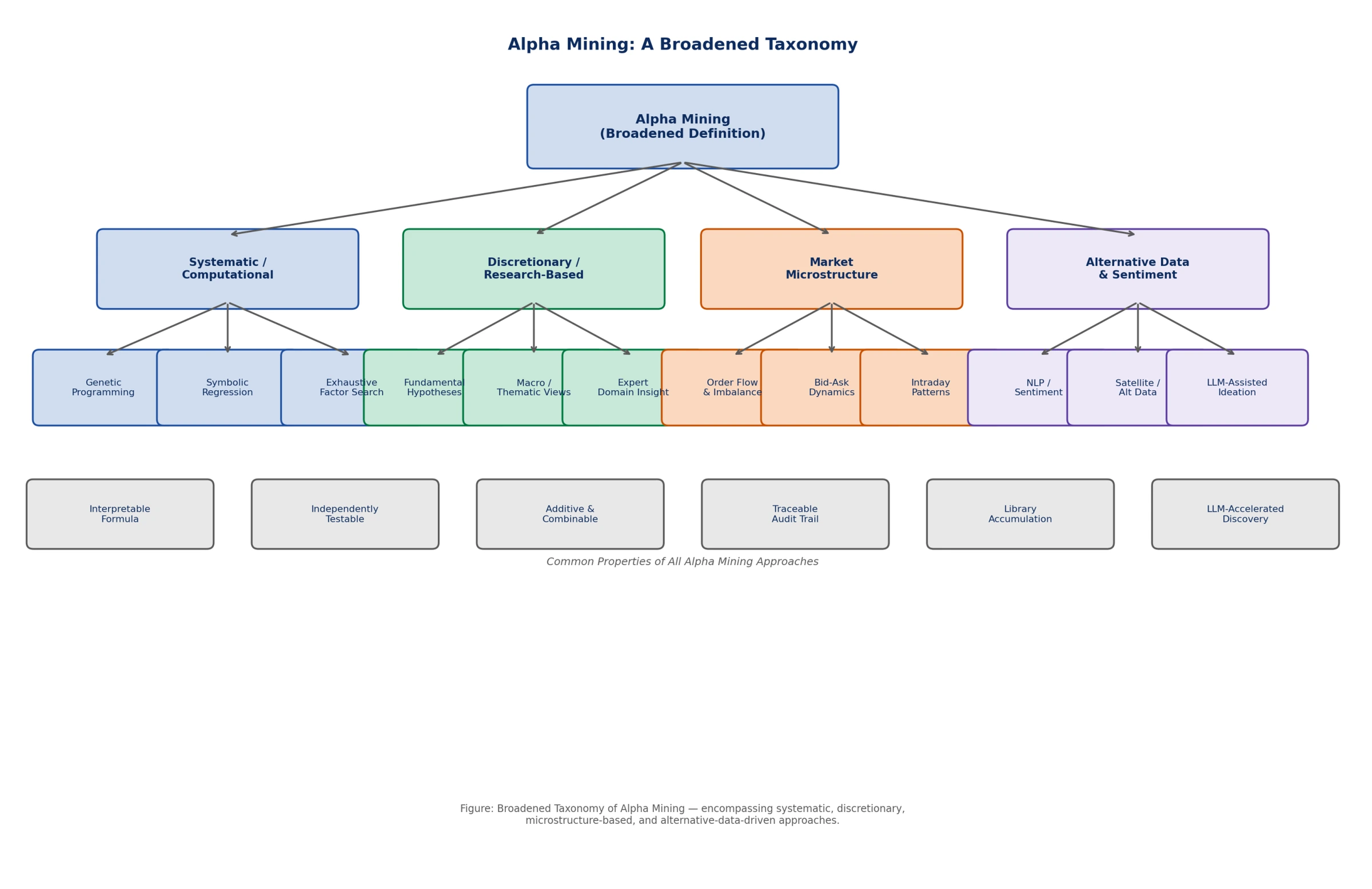
Figure 1 — Broadened taxonomy of alpha mining approaches. The four pillars— systematic/computational, discretionary/research-based, market microstructure, and alternative data & sentiment—all share the same defining properties: interpretable formula, independent testability, additive combinability, and traceable audit trail.

2.1.1 Systematic / Computational Alpha Mining

The most widely studied branch employs automated search over large spaces of candidate signal expressions. Genetic programming evolves operator trees applied to price, volume, and fundamental data; symbolic regression fits compact mathematical expressions to return cross-sections; and exhaustive factor search evaluates pre-specified transformations across a combinatorial grid. The output is a signal formula with a closed-form expression that can be independently evaluated and backtested.

2.1.2 Discretionary and Research-Based Alpha Mining

Not all mined alphas originate from automated search. A substantial fraction of production alphas in top-tier quantitative funds originate from discretionary hypothesis formulation: an experienced researcher observes a market phenomenon, articulates an economic mechanism, operationalizes it as a quantitative signal, and validates it through rigorous statistical testing. Examples include earnings revision signals derived from analyst behavior theory, insider ownership signals derived from principal-agent considerations, and supply-chain contagion signals derived from sector-level economic reasoning. This branch also encompasses macro and thematic views that are operationalized as quantitative signals: a researcher who believes that central bank policy shifts create systematic mispricing in rate-sensitive equities can formulate and test a signal that captures this relationship, even if the signal was not discovered by an automated search process. The key requirement is that the signal be independently testable and additive—not that it originated from a computer.

2.1.3 Market Microstructure-Based Alpha Mining

A distinct and often underappreciated category of alpha mining exploits the mechanics of price formation rather than fundamental or macro variables. Microstructure signals derive from:

• Order flow and imbalance: persistent directional imbalance between buyer-initiated and seller-initiated trades predicts short-term price movements, reflecting informed trading activity;
• Bid-ask dynamics: changes in the spread, depth at the best bid and ask, and queue composition carry information about short-term supply and demand;
• Intraday patterns: time-of-day effects, opening auction dynamics, and closing fixings create predictable price patterns that can be exploited by signals calibrated on intraday data. Microstructure alphas are particularly important because they are naturally orthogonal to fundamental and macro signals, providing diversification within the alpha library. They also tend to decay more slowly than pure price-based momentum signals, because their source—the mechanics of price formation—is structural rather than behavioral.

2.1.4 Alternative Data and Sentiment Alpha Mining

The most recent pillar of alpha mining exploits data sources that lie outside traditional market and fundamental data: satellite imagery of retail parking lots, credit card transaction flows, web traffic to corporate websites, natural language feeds from earnings calls and news, and social media sentiment. These data sources are operationalized as quantitative signals through standard statistical methods (regression, classification) or through more sophisticated NLP pipelines. The emergence of LLM-assisted ideation has transformed this category: agentic LLMs can now generate, implement, and backtest alternative data signals at a rate that far exceeds human researcher capacity, dramatically expanding the hypothesis space and accelerating the discovery pipeline [2].

2.1.5 Common Properties Across All Branches

Despite their methodological diversity, all four branches share the defining properties of alpha mining:

1. (i) Interpretability: the signal has a human-readable functional form or economic rationale;

(ii) Testability: the signal can be evaluated in isolation via a well-defined backtest protocol; (iii) Additive combinability: the signal contributes incrementally to a portfolio when combined with existing alphas, subject to correlation constraints;

(iv) Auditability: the signal’s source, derivation, and validation history are traceable;

1. (v) Library accumulation: discovered signals are stored in a persistent, queryable library that constitutes the fund’s institutional memory.

2.2 From Raw Alphas to Signals to Portfolios

The preceding subsections describe what alphas are and where they come from. This subsection formalises the missing link: how individual alpha expressions are aggregated into tradeable portfolio weights. The pipeline has three sequential stages.

Stage 1 — Signal Normalisation An alpha expression produces a raw scalar score 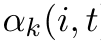) for instrument i at time t. Raw scores are not directly combinable because they live on different scales and may have nonstationary distributions. Two standard normalisations are applied:

• Cross-sectional rank normalisation:

where is the universe size at time t. Robust to outliers and non-stationarity.

• Cross-sectional z-scoring:

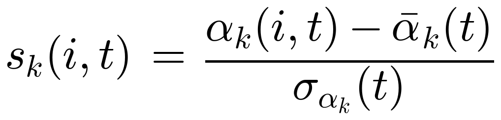
preserving cardinal distances when signal magnitude carries information.

Each signal is then factor-neutralised to remove common factor exposures that would otherwise make the composite alpha a disguised bet on crowded premia:

where is the factor exposure matrix (sector dummies, Barra-style style factors). The residual k is the idiosyncratic signal component orthogonal to the crowded factor space.

A decay multiplier 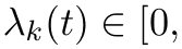1], derived from the trailing Information Coefficient half-life of alpha k, scales each signal:

When the IC has decayed below a threshold (monitored by the half-life detection subsystem described in Section 10), 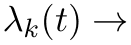0 and the alpha is effectively retired from the combination. Stage 2 — Composite Alpha Construction With K normalised, decay-adjusted, neutralised signals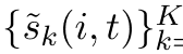 , the portfolio-of-signals problem finds combination weights such that:

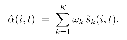
Three approaches are used in practice:

(1) IC-weighted / ICIR: weight each signal by its trailing Information Ratio, IC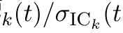), penalising signals with high average IC but unstable IC across regimes—directly addressing the overfitting and regime-sensitivity concerns discussed in Section 4.

(2) Mean-variance optimisation over signals: treat the combination as a QP,

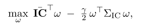
where ΣIC is the covariance matrix of IC time series across signals. Exploits low-correlation signals and down-weights redundant ones.

(3) LASSO regression: for large alpha libraries (K in the hundreds, as enabled by LLM-assisted hypothesis generation), penalisation produces a sparse ˆω that automatically selects non-redundant signals and directly addresses the alpha crowding problem. Stage 3 — Portfolio Construction via the Optimizer Layer The composite alpha vector ˆ 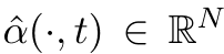is the return forecast ˆµ that enters the portfolio optimizer layer described in Section 10. The optimizer solves:

subject to turnover, leverage, factor neutralisation, and position limit constraints. The complete pipeline is therefore:

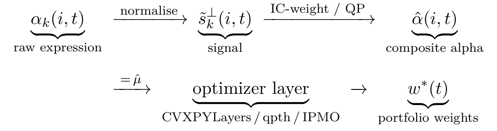
This explicit, auditable pipeline is the alpha mining paradigm’s primary explainability advantage: every component of ˆµ can be traced back to a specific with a known weight and a monitored IC history. Deep learning systems collapse this entire pipeline into a single jointly-optimised mapping—gaining end-to-end gradient alignment at the cost of that transparency.

2.3 Deep Learning Alpha Generation

We define deep learning alpha generation as any process in which a parameterized neural network learns to map a high-dimensional input feature matrix—comprising price, volume, fundamental, alternative, and sentiment data—directly to return predictions, portfolio weights, or trading actions, without requiring the practitioner to prespecify the functional form of the predictive relationship.

The defining properties of a DL alpha system are:

1. (i) End-to-end learning: feature interactions are discovered by the model, not pre-specified;

(ii) Dynamic weighting: the model can implicitly vary the importance of features across time, regime, and instrument;

(iii) High capacity: the model can represent nonlinear, long-range, and cross-sectional dependencies that are inaccessible to linear factor models;

(iv) Opacity: the model’s predictions are not directly interpretable without auxiliary explainability tools.

The primary architectures in current use are Transformers (which use multihead self-attention to model long-range temporal and cross-sectional dependencies) and LSTMs (which use gated recurrent units to model sequential dependencies with explicit memory). Hybrid and hierarchical combinations of these architectures are increasingly common in production systems.

2.4 Scope and Assumptions

This analysis focuses on medium-frequency strategies (holding periods from minutes to weeks) where both paradigms are actively competitive. We do not address ultra-high-frequency market-making (where latency dominates) or purely fundamental long-horizon investing (where deep learning has limited applicability). We assume institutional-grade infrastructure and data access for both paradigms, and we evaluate both from the perspective of a well-resourced quantitative fund operating in 2025–2026.

3 Alpha Research Sustainability

3.1 Resource and Compute Profile

Systematic alpha mining is computationally intensive during the discovery phase—genetic programming over large universes can require substantial compute—but is lightweight in production: a library of linear or low-complexity signals can be evaluated and combined in milliseconds on commodity hardware. The ongoing resource requirement is proportional to the rate of new alpha discovery, which can be modulated.

Deep learning systems invert this profile. Training a Transformer on multi-year, multi-asset feature matrices requires GPU clusters; inference is faster but still demands dedicated hardware for real-time feature computation and model serving. Critically, the resource requirement is recurring: models must be periodically retrained as market conditions evolve, and each retraining cycle is as expensive as the original—a structural cost that compounds over time.

Key Insight 1. For organizations without sustained access to large-scale GPU infrastructure and high-quality alternative data pipelines, systematic alpha mining offers a more sustainable resource profile. For well-resourced firms, DL’s recurring costs are offset by the breadth and depth of signals it can discover.

3.2 Data Requirements

Systematic pipelines can extract value from smaller, curated datasets because domain knowledge constrains the hypothesis space. A researcher who hypothesizes a specific earnings-revision signal needs only the relevant earnings data, not a complete feature matrix.

DL systems are data-hungry by construction: their expressive power is only realized when the training set is large enough to prevent overfitting. In practice, this means that DL systems benefit disproportionately from data breadth—more instruments, more features, longer histories—and from alternative data (satellite imagery, credit card transactions, natural language feeds) that is expensive to acquire and process [10].

3.3 Regulatory and Explainability Pressures

Regulatory trends in major jurisdictions are moving toward greater model transparency and auditability. The EU AI Act and analogous frameworks in the US and UK impose explainability requirements on algorithmic decision-making systems in financial services. Systematic pipelines, which produce interpretable signals with traceable economic rationale, are structurally better positioned to satisfy these requirements.

DL systems can be made more explainable through auxiliary tools (SHAP values, layerwise relevance propagation, attention visualization), but these tools produce post-hoc approximations of model behavior rather than genuine interpretability. Regulatory acceptance of post-hoc explainability remains uncertain and jurisdiction-dependent [11].

3.4 Innovation Pace and Tooling Ecosystem

The tooling ecosystem for systematic alpha mining is mature: open-source libraries for genetic programming (DEAP, gplearn), factor testing (Alphalens, QuantLib), and portfolio construction (Riskfolio-Lib, PyPortfolioOpt) are well-developed and widely adopted. LLM-assisted hypothesis generation represents the most significant recent innovation, dramatically accelerating the ideation phase [2].

DL tooling is evolving rapidly but remains more specialized: experiment tracking (MLflow, Weights & Biases), distributed training (PyTorch Distributed, DeepSpeed), and financial-specific frameworks (FinRL, Qlib) require dedicated ML engineering resources. The pace of innovation in DL is faster, but the operational complexity is correspondingly higher.

4 Neural Network Trading Robustness

4.1 Overfitting: Failure Modes and Detection

Overfitting is the central robustness challenge for both paradigms, but the failure modes are qualitatively different.

In systematic alpha mining, overfitting manifests as backtest mining bias: a signal that appears statistically significant in-sample due to multiple testing across a large search space. This failure mode is well-understood and has well-developed mitigations: the Deflated Sharpe Ratio (DSR) [4], the Combinatorially Symmetric Cross-Validation (CSCV) framework [5], and Bonferroni-style corrections for multiple comparisons. Crucially, because each alpha is independently testable, overfitting can be detected and corrected at the signal level before portfolio assembly.

In deep learning systems, overfitting is more insidious. A Transformer trained on historical market data can memorize complex, high-order patterns that are specific to the training period without these patterns being detectable through standard metrics. The model may report excellent in-sample performance while having learned spurious correlations that do not generalize. Detection requires adversarial testing frameworks that estimate the probability of backtest overfitting and reject candidate DRL agents whose performance is inconsistent with genuine predictive skill.

4.2 Regime Changes

Both paradigms are vulnerable to regime changes, but the nature of the vulnerability differs. Systematic mining responds to regime changes at the signal level: individual alphas decay at different rates, and the portfolio-of-signals framework provides natural diversification across regime sensitivities. When a regime shift is detected, the practitioner can surgically downweight or retire signals that are regime-specific while retaining those that are regime-agnostic. This modularity is a significant robustness advantage.

DL systems face regime changes as a distributional shift problem: the joint distribution of features and returns changes, and a model trained on the old distribution may produce biased predictions. Mitigations include:

• Regime-aware architecture search (RegimeNAS): differentiable neural architecture search with regime-specific blocks (volatility, trend, and range modules) and Lipschitz stability penalties that constrain the model’s behavior during transitions [6];
• Invariant feature learning: methods that separate environment-agnostic features (persistent signals) from environment-specific features (regime-dependent signals), retaining the former and adapting the latter [7];
• Online and continual learning: architectures designed for continuous parameter updates as new data arrives, avoiding the need for full retraining cycles [8];
• Adversarial training with synthetic regimes: macro-conditioned generative simulators that expose the model to diverse, plausible regime scenarios during training, narrowing the gap between in-sample and out-of-sample performance [9].

4.3 Alpha Decay

Alpha decay—the gradual erosion of a signal’s predictive power as it becomes known and arbitraged—affects both paradigms but with different dynamics.

In alpha mining, decay is gradual and renewable: individual signals decay as they are discovered and traded by competitors, but the discovery process continuously generates new signals. The alpha library is a living repository that can be replenished. Practitioners monitor each signal’s live Sharpe ratio against its backtest estimate and apply a “decay haircut” to forward performance expectations.

In DL systems, decay is potentially catastrophic and sudden: if the model’s learned representations are heavily concentrated in a small number of high-capacity features that become crowded, performance can collapse abruptly rather than gradually. However, DL systems with well-designed cold-storage libraries (discussed in Section 10) can mitigate this by maintaining versioned model snapshots that can be reactivated when market conditions return to states that favor earlier representations.

Empirical evidence from Transformer-based factor generation suggests that learned factors exhibit longer half-lives and lower turnover than many short-lived linear factors [15], consistent with the hypothesis that DL models can discover more structurally persistent patterns when properly regularized.

4.4 Out-of-Sample Generalization

A consistent finding in the literature is that simpler models with explicit regularization often produce smaller out-of-sample generalization gaps than large neural networks trained end-to-end [22]. GBDTs with dropout and post-prediction neutralization frequently outperform Transformers on standard equity prediction benchmarks when the training set is modest. This finding should not be interpreted as evidence against DL, but rather as a reminder that DL’s advantages are conditional: they require sufficient data, appropriate regularization, and regime-aware validation to materialize. In data-rich environments with well-engineered pipelines, DL systems can and do achieve superior generalization [21].

5 Competitive Moat

5.1 Sources of Moat in Alpha Mining

The competitive moat in alpha mining derives from four sources:

1. (1) Alpha library depth: a large, well-curated library of independent signals, accumulated over years of disciplined research, is difficult to replicate. The library’s value is not in any individual signal—which may be discoverable by a competitor—but in the combination of hundreds of low-correlation signals that collectively produce a stable, high-Sharpe portfolio. The library also encodes negative knowledge: signals that were tested and rejected, preventing redundant exploration.
2. (2) Process institutional knowledge: the research process—hypothesis generation, testing protocols, debiasing procedures, signal combination methodology—is embedded in organizational culture and is not fully transferable. This process knowledge is a durable moat that erodes slowly.
3. (3) Proprietary data: unique data sources (proprietary order flow, alternative data partnerships, exclusive data cleaning pipelines) increase the replication cost for competitors [13].
4. (4) Continuous discovery: the ability to continuously generate new alphas as existing ones decay ensures that the library remains current. LLM-assisted hypothesis generation has dramatically accelerated this process, giving well-resourced systematic shops a significant speed advantage [2]. The primary vulnerability of systematic moats is signal crowding: as more participants discover and trade the same factors, the associated returns are arbitraged away. Public factor discoveries (momentum, value, quality, low volatility) have experienced significant decay since their publication [12], and the growing use of LLMs for hypothesis generation may accelerate this process by homogenizing the discovery landscape.

5.2 Sources of Moat in Deep Learning Systems

The competitive moat in DL systems is structurally different and, we argue, compounding over time in ways that alpha mining moats are not. The sources are:

1. (1) Proprietary data pipelines: DL systems are uniquely dependent on large, diverse, highquality datasets. A firm that has invested years in building proprietary data acquisition, cleaning, and normalization pipelines has a moat that is extremely difficult to replicate, because the value is embedded in the process of data production, not just the data itself.
2. (2) Architectural recipes: the specific combination of architecture choices, training hyperparameters, regularization techniques, and ensemble configurations that produce a well-performing DL system is a form of tacit knowledge that is not revealed by the model’s outputs. Competitors cannot reverse-engineer the recipe from observing the fund’s trades.
3. (3) Training compute history: DL models benefit from curriculum learning—training on progressively harder examples—and from transfer learning from related tasks. A firm that has accumulated years of training compute history and model checkpoints has a head start that cannot be quickly replicated by a new entrant, regardless of their current compute budget.

(4) Strategy cold-storage libraries: analogous to alpha libraries in alpha mining, well-engineered DL shops maintain versioned repositories of trained model snapshots, each associated with the market conditions and data distribution under which it was trained. These libraries can be queried to reactivate models that performed well in historical regimes similar to current conditions, providing a form of institutional memory that compounds with time (Section 10).

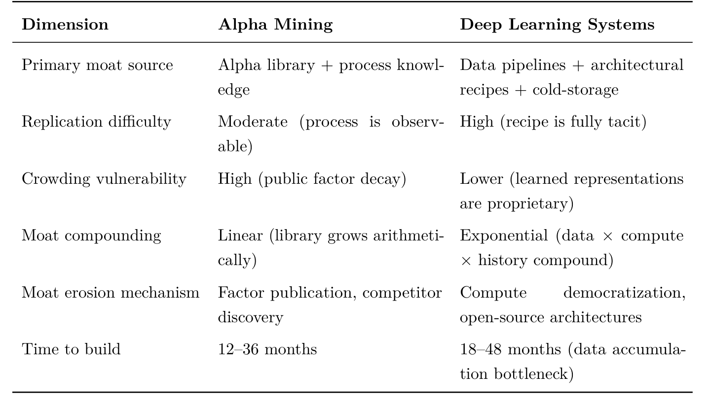
Key Insight 2. The DL moat is a systems moat, not a model moat. It derives from the accumulation of proprietary data, training history, architectural recipes, and cold-storage libraries—none of which are revealed by the model’s outputs and none of which can be quickly replicated. This moat compounds as the system accumulates more data, more training history, and more model snapshots.

5.3 Comparative Moat Durability

6 Technological and Compute Moats

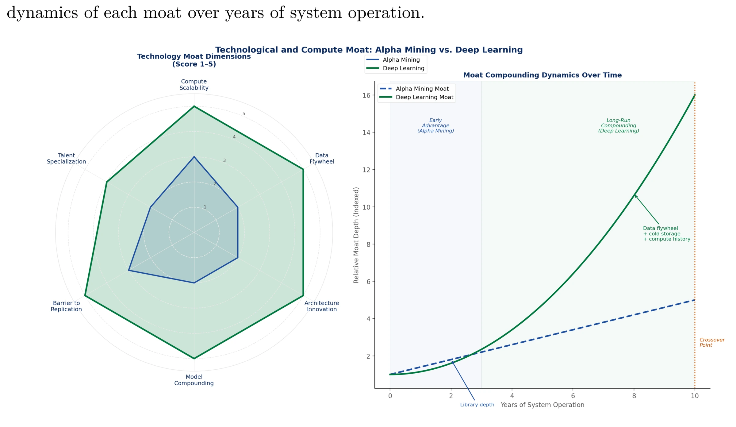
Beyond the signal-level and process-level moats discussed in the previous section, a distinct and increasingly decisive competitive dimension is the technological and compute moat: the degree to which a firm’s technology stack, infrastructure investment, and accumulated compute history constitute barriers to replication that are independent of any specific signal or model. This section argues that deep learning systems have a structurally higher long-run advantage on this dimension—in both moat depth and strategy efficacy—than alpha mining approaches.

Figure 2 — illustrates this argument across two complementary views: a radar chart comparing the two paradigms across six technology moat dimensions, and a time-series showing the compounding dynamics of each moat over years of system operation.

6.1 Architecture Innovation and the Research Compounding Effect

Of all the technological moat dimensions, architecture innovation is the most decisive. In alpha mining, the research process produces signals stored in a library; each new signal is an independent addition and signals do not interact to improve the discovery of future signals (beyond the negative knowledge of tested-and-rejected hypotheses).

In deep learning, architectural innovations compound multiplicatively: a new regularization technique (e.g., Lipschitz constraints) improves all future models trained with it; a new training procedure (e.g., curriculum learning) improves the utilization of all historical data; a new architecture (e.g., RegimeNAS) improves performance across all market regimes simultaneously. The research team’s accumulated understanding of what works—embedded in training recipes, data preprocessing pipelines, and model architectures—constitutes a form of tacit technological knowledge that is not transferable and not replicable from first principles.

This creates a research compounding effect: each architectural improvement multiplies the value of all existing data and compute, whereas in alpha mining, each new signal adds value arithmetically. Critically, this compounding begins immediately—a team with strong architectural intuition can build a meaningfully differentiated system within 6–12 months, well before data flywheels or cold-storage libraries have had time to accumulate.

6.2 Model Compounding and the Cold-Storage Advantage

The second primary moat driver is model compounding via cold-storage. As detailed in Section 10, DL systems that maintain cold-storage libraries of trained model snapshots accumulate a form of institutional memory that has no direct analogue in alpha mining. The key point from a technology moat perspective is that this library compounds in value as the system experiences more market regimes:

• After 6–12 months: the library contains models trained on diverse intraday and short-cycle regimes;
• After 18–24 months: the library spans at least one full market cycle, enabling regimeconditional model reactivation;
• After 3–5 years: the library contains multiple full cycles with regime-specific snapshots that can be activated when historical conditions recur. A new DL competitor, regardless of their current compute budget, cannot acquire this historical model library without experiencing those market cycles. The cold-storage moat is therefore time-locked: it cannot be purchased, only accumulated.

6.3 Compute Scalability and the GPU Cluster Moat

Alpha mining is computationally bounded: the primary compute requirement is the backtest engine, which scales linearly with the number of candidate signals and the length of the historical window. Beyond a certain scale, additional compute produces diminishing returns in signal discovery. Deep learning systems have no such ceiling. Additional compute enables:

• Larger models: Transformer architectures scale with compute in a well-documented power-law relationship; larger models trained on more data consistently outperform smaller models in prediction tasks [10];
• More frequent retraining: with sufficient compute, models can be retrained daily or even intraday, maintaining alignment with current market dynamics;
• Broader architecture search: differentiable NAS over larger search spaces finds better architectures, and this search scales with compute;
• Richer simulation: adversarial training with macro-conditioned synthetic market generators requires substantial compute but produces measurably more robust models [9]. A firm that has invested in a large GPU cluster not only has better models today but has a structural infrastructure advantage that cannot be quickly replicated by a competitor without equivalent capital expenditure.

6.4 Barrier to Replication and Talent Specialization

The combination of proprietary data pipelines, architectural recipes, training compute history, and cold-storage libraries creates a barrier to replication that is qualitatively higher than that of alpha mining. A competitor who observes a systematic fund’s trades can, in principle, reverse-engineer many of its signals through careful analysis. A competitor who observes a DL fund’s trades cannot reverse-engineer its architecture, training procedure, data pipeline, or model weights—the moat is fully tacit. The talent requirement is also higher and more specialized: DL systems require ML engineers, data engineers, MLOps specialists, and quantitative researchers working in close collaboration. This talent combination is scarce and expensive, and the institutional knowledge embedded in the team is itself a moat component.

6.5 The Data Flywheel Effect (Supporting Factor)

A secondary, longer-horizon moat is the data flywheel: a self-reinforcing cycle in which more data enables better models, which generate better predictions, which attract more capital and data partnerships, which produce more data. While real, this effect is slower to materialize than architecture innovation or model compounding—it typically requires 2–4 years of live operation before the proprietary data asset becomes a meaningful differentiator. In alpha mining, additional data improves signal discovery at a diminishing marginal rate but does not create a compounding feedback loop, so the flywheel advantage is DL-specific. However, practitioners should not overweight this factor in near-term moat assessments; architectural and model compounding advantages manifest far sooner.

6.6 Long-Run Efficacy: Why Compute Advantage Translates to Alpha

The technology moat argument would be incomplete without addressing whether compute advantage translates to alpha generation efficacy, not just replication difficulty. The argument for long-run DL efficacy superiority rests on three structural claims:

1. (1) Nonlinearity capture: as markets become more complex—more participants, more data sources, more interconnected feedback loops—the predictive value of nonlinear, high-dimensional models relative to linear factor models increases. The increasing complexity of markets is a secular trend that favors DL’s architectural strengths;
2. (2) Alternative data exploitation: the volume and variety of alternative data sources is growing exponentially. DL systems are uniquely capable of ingesting and learning from high-dimensional, heterogeneous alternative data (text, images, time-series, graph data) in a unified framework; alpha mining requires each data source to be operationalized into a discrete signal, which is a bottleneck that does not exist for DL;
3. (3) Adaptive learning: markets are adversarial environments in which strategies are arbitraged away as they become known. DL systems that can continuously adapt their learned representations have a structural advantage in this adversarial environment over alpha mining approaches that rely on fixed signal formulas. These three claims collectively support the conclusion that, in the long run, DL systems operating with sustained compute investment will generate higher risk-adjusted returns than alpha mining approaches operating on equivalent data—provided that the DL systems are engineered with the robustness mechanisms described in Section 10.

7 Market Regime Adaptability

7.1 Regime Taxonomy

We distinguish four market regime types relevant to this comparison:

(I) Trending regimes: sustained directional price movement driven by fundamental or macro factors;

(II) Mean-reverting regimes: high-frequency oscillation around equilibrium, driven by market microstructure and behavioral overcorrection;

(III) Volatility regimes: periods of elevated or depressed realized volatility, often associated with macro uncertainty or liquidity crises;

(IV) Behavioral/sentiment regimes: periods dominated by retail herding, momentum cascades, or policy-driven sentiment shifts.

7.2 Systematic Mining Under Regime Shifts

Systematic mining handles regime shifts through signal-level diversification: a well-constructed alpha library contains signals that are differentially sensitive to each regime type. Momentum signals perform in trending regimes; mean-reversion signals perform in oscillating regimes; volatility signals hedge across regimes. The portfolio-of-signals framework naturally diversifies across regime sensitivities, provided the library is sufficiently broad.

The limitation is that alpha mining assumes stationarity within regimes: each signal is assumed to have a stable predictive relationship within a given regime type. When this assumption breaks—when the nature of a regime changes in ways that are not captured by the signal’s functional form—the signal decays without providing a mechanism for adaptation.

7.3 Deep Learning Under Regime Shifts

DL systems can, in principle, adapt to regime shifts more fluidly because their learned representations are not fixed functional forms. A Transformer that has been trained on data spanning multiple regimes can learn to identify regime-indicative patterns in its input features and adjust its predictions accordingly—without requiring the practitioner to explicitly specify the regime taxonomy.

This advantage is most pronounced in behavioral and sentiment regimes, where the predictive patterns are high-dimensional, nonlinear, and not easily captured by interpretable signals. In trending and mean-reverting regimes, the advantage is more modest, because these regimes are well-described by simple momentum and reversion signals that alpha mining handles effectively. The key enablers of DL’s regime adaptability are:

• Multi-head attention: allows the model to simultaneously attend to multiple time scales and feature types, naturally weighting different inputs as their predictive relevance changes across regimes;
• Regime-aware architecture search: RegimeNAS-style systems that route inputs to specialized blocks based on detected regime state [6];
• Invariant learning: methods that separate regime-agnostic from regime-specific features, ensuring that the model retains persistent signals while adapting regime-sensitive components [7].

8 Agentic LLM Integration

8.1 The Agentic LLM Paradigm

Agentic LLMs—large language models equipped with tool-use capabilities, memory, and multi-step reasoning—represent a qualitatively new capability for quantitative research workflows. Unlike earlier NLP applications (sentiment scoring, news classification), agentic LLMs can autonomously execute research pipelines: formulating hypotheses, writing and running code, interpreting results, and iterating based on feedback [2].

8.2 Fit with Systematic Alpha Mining

Agentic LLMs are a natural accelerant for systematic alpha mining, because the mining process is inherently linguistic and iterative:

• Hypothesis generation: LLMs can generate hundreds of economically motivated factor hypotheses per hour, dramatically expanding the hypothesis space beyond what a human researcher can explore [2];
• Expression synthesis: LLMs can translate natural-language hypotheses into formal mathematical expressions suitable for backtesting, bridging the gap between economic intuition and quantitative implementation;
• Human-in-the-loop refinement: reflective agent architectures allow LLMs to receive feedback on backtest results and iteratively refine signal specifications without retraining a neural network [20];
• Documentation and governance: LLMs can automatically generate human-readable descriptions of each alpha, its economic rationale, and its validation history, improving auditability and regulatory compliance;
• Crowding detection: LLMs can monitor the academic literature and competitor disclosures to identify signals that are becoming crowded, triggering preemptive retirement from the production library.

8.3 Fit with Deep Learning Systems

Agentic LLMs play a more peripheral role in DL systems, because the core learning process— neural network training—is not amenable to linguistic iteration. However, LLMs can contribute in several auxiliary capacities:

• Feature engineering: LLMs can suggest and implement novel feature transformations that enrich the input feature matrix, improving the signal-to-noise ratio for the downstream model;
• Architecture search: LLMs can assist in exploring the hyperparameter and architecture space, though this role is increasingly automated by differentiable NAS systems;
• Post-hoc interpretation: LLMs can synthesize SHAP or LRP attribution outputs into human-readable explanations, supporting governance and risk review;
• Monitoring and alerting: LLMs can monitor live model performance metrics and generate natural-language summaries of anomalies, accelerating the human response to regime shifts.

Key Insight 3. Agentic LLMs are a force multiplier for systematic alpha mining—they can accelerate every stage of the discovery lifecycle. For DL systems, they are a useful but peripheral tool, contributing primarily to auxiliary tasks rather than the core learning process.

9 Market Case Studies: Structure Determines Paradigm Advantage

The following case studies are presented not as primary evidence for either paradigm, but as illustrations of how market microstructure determines which paradigm is structurally advantaged. The central thesis is that DL’s advantages are proportional to the degree of nonlinearity, behavioral complexity, and non-stationarity in the market environment.

9.1 Chinese A-Share Equities

Chinese A-share markets present a unique microstructural environment characterized by several features that collectively favor DL architectures: Retail dominance: retail investors account for approximately 70–85% of daily trading volume in A-shares, compared to 15–25% in US equity markets. This structural fact is not mitigated by trading restrictions (T+1 settlement, 10% daily price limits), which disproportionately constrain institutional participants while leaving the retail segment’s aggregate volume largely unaffected. The result is a market dominated by behavioral, momentum-chasing, and herding dynamics that are nonlinear and rapidly rotating. Policy sensitivity: Chinese equity markets are unusually sensitive to government policy announcements, regulatory interventions, and macroeconomic signaling from state institutions. These policy shocks create abrupt, nonlinear regime transitions that are difficult to capture with linear factor models calibrated on stable historical relationships.

Reversal dynamics: empirical studies document strong short-cycle reversal effects in A-shares, driven by retail overcorrection and behavioral cascades [14]. These reversal patterns are high-frequency, nonlinear, and regime-dependent—precisely the type of signal that Transformer architectures are designed to capture. Factor crowding: as the Chinese quant industry has grown, linear factor premia (momentum, value, size, quality) have experienced rapid crowding, with factor returns declining as more capital chases the same signals. DL systems, which learn proprietary, high-dimensional representations, are less susceptible to this crowding because their learned features are not publicly observable. Empirical backtest evidence supports the structural argument: Transformer-based factor generation on 4,601 Chinese stocks (2010–2019) outperformed 100 factor-based strategies while producing lower turnover and longer factor half-lives [15]. Multi-source Transformer models combining Time2Vec encoding with heterogeneous data inputs outperformed MLP, SVM, GBDT, LSTM, and attention-LSTM baselines on CSI300 and A50 samples [16].

9.2 Commodity Futures

Commodity futures markets occupy an intermediate position in the paradigm comparison. They share several features with A-shares—retail speculative participation (especially in Chinese commodity futures), sentiment-driven price action, and nonlinear supply-demand dynamics—but also have a fundamental anchor absent in equity markets: physical supply and demand, storage costs (the cost-of-carry relationship), and geopolitical supply shocks create partially predictable structural regimes. This dual nature implies a frequency-dependent paradigm advantage:

• At medium-to-long horizons (weeks to months), systematic alpha mining retains competitive advantage through carry signals (roll yield), momentum, and supply-demand fundamentals that are structurally persistent;
• At short horizons (intraday to days), DL architectures are advantaged by their ability to model the nonlinear, sentiment-driven, and microstructure-dependent dynamics that dominate short-cycle price movements. The practical implication is that commodity futures strategies benefit from hybrid architectures: a systematic foundation (carry, momentum, fundamentals) augmented by a DL layer that captures short-cycle behavioral dynamics and regime transitions.

9.3 Cryptocurrency Markets

Cryptocurrency markets represent the extreme case of DL structural advantage. The features that favor DL in A-shares are present in cryptocurrency to an even greater degree:

• Extreme retail dominance: institutional participation in cryptocurrency markets remains limited, and retail sentiment—amplified by social media, influencer dynamics, and narrative cycles—is the primary driver of price action;
• No fundamental anchor: unlike equities (earnings, book value) or commodities (supplydemand fundamentals), most cryptocurrencies have no fundamental valuation anchor, making price dynamics almost entirely sentimentand momentum-driven;
• 24/7 continuous trading: the absence of market closes, circuit breakers, and trading restrictions eliminates the behavioral dampening that these mechanisms provide in traditional markets;
• Extreme non-stationarity: cryptocurrency markets have experienced multiple full regime cycles (bull, bear, sideways, crisis) within short historical windows, making stationarity assumptions untenable;
• High turnover and velocity: cryptocurrency turnover ratios dwarf those of any traditional asset class, creating a rich, high-frequency behavioral signal that DL architectures can exploit. For cryptocurrency markets, linear alpha mining faces a fundamental challenge: the absence of a stable factor structure means that discovered signals decay extremely rapidly as market dynamics evolve. DL systems, which can adapt their learned representations to changing dynamics, are structurally better suited to this environment.

9.4 Synthesis: The Market-Structure Principle

The three case studies support a general principle that we term the Market-Structure Principle: Market-Structure Principle: The relative advantage of deep learning over systematic alpha mining is proportional to the degree of (a) retail/behavioral participation, (b) nonlinearity and non-stationarity in price dynamics, (c) absence of fundamental anchors, and (d) factor crowding in the linear factor space. Markets with high scores on all four dimensions (cryptocurrency) favor DL strongly; markets with low scores (institutional equity in developed markets) favor alpha mining; intermediate markets (commodity futures, A-shares) favor hybrid approaches.

10 Why Deep Learning Strategies Develop Deeper Moats Over Time

This section develops the central argument of the paper: that well-engineered DL systems, unlike vanilla neural network implementations, compound their competitive moat over time through a set of architectural and operational mechanisms that have no direct analogue in systematic alpha mining. The key mechanisms are: (1) strategy cold-storage libraries, (2) portfolio optimizer layers, (3) adaptive trading mechanism layers, (4) overfitting and alpha-decay mitigation systems, and (5) regime-aware architecture compounding.

10.1 Strategy Cold-Storage Libraries

The most underappreciated source of compounding moat in DL systems is the strategy cold-storage library: a versioned repository of trained model snapshots, each tagged with the market conditions, data distribution, and performance characteristics of the period in which it was trained. The analogy with systematic alpha mining is precise but the mechanism is different. In alpha mining, the alpha library stores signal formulas—interpretable expressions that can be re-evaluated on current data. In DL cold storage, the library stores trained model weights— parameterized representations of learned market dynamics that can be reactivated when current market conditions resemble the conditions under which the model was trained. The cold-storage library enables several capabilities:

• Regime-matched model selection: given current market conditions (characterized by volatility, correlation structure, sentiment indicators, and macroeconomic state), the system queries the cold-storage library to identify historical periods with similar characteristics and activates the model snapshot trained on those periods;
• Ensemble construction: multiple model snapshots from different historical periods can be combined in an ensemble, with weights determined by the similarity between their training conditions and current conditions;
• Catastrophic forgetting prevention: by maintaining snapshots of models trained on earlier market regimes, the system avoids the catastrophic forgetting problem that afflicts continually retrained models—the ability to perform well in current conditions while losing the ability to perform in historical regimes;
• Institutional memory accumulation: the cold-storage library grows with every market cycle, encoding an increasingly comprehensive map of market dynamics that a new entrant cannot replicate without experiencing those cycles.

The compounding nature of this moat is critical: each market cycle adds new model snapshots to the library, increasing its coverage and depth. A firm that began building its cold-storage library in 2015 has experienced multiple full market cycles (2018 correction, 2020 COVID crash, 2022 rate shock, 2024–2026 AI-driven volatility) and has model snapshots trained on each. A new entrant in 2026 cannot acquire this history regardless of its current compute budget.

10.2 Portfolio Optimizer Layers

A vanilla DL system produces return predictions or ranking scores for individual instruments. Translating these predictions into a live portfolio requires a portfolio optimizer layer that accounts for transaction costs, risk constraints, factor neutralization, and position limits. The design of this layer is a significant source of differentiation.

10.2.1 Architecture of the Portfolio Optimizer Layer

A well-engineered portfolio optimizer layer consists of the following components:

1. (1) Return prediction module: the base Transformer or LSTM model produces a vector of expected returns ˆ 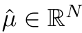for N instruments, along with a predictive uncertainty estimate ˆ 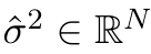from variational or distributional output heads;
2. (2) Covariance estimation module: a separate model (or the same model with appropriate output heads) estimates the 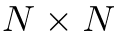covariance matrix ˆΣ of returns, incorporating both factor-model structure and residual correlations;
3. (3) Factor neutralization layer: the predicted returns are projected onto the null space of a factor exposure matrix 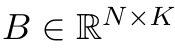(where K is the number of common factors), producing factor-neutral alpha signals ˆ; 2ˆΣw subject to
4. (4) Mean-variance optimization: the optimizer solves maxˆ constraints on turnover, leverage, and position limits, where λ is a risk-aversion parameter;
5. (5) Transaction cost model: a learned model of market impact and bid-ask spread that adjusts the optimization objective to account for the cost of executing the target portfolio;
6. (6) Kelly-like position sizing: for strategies with well-calibrated probability estimates, Kellyfractional position sizing can be applied to maximize long-run growth rate, as demonstrated in LSTM-based systems with dynamic K-top selection [17]. The key insight is that the portfolio optimizer layer is itself learnable: the covariance model, the transaction cost model, and the factor exposure matrix can all be parameterized and trained jointly with the base prediction model, producing an end-to-end system that optimizes for realized portfolio performance rather than prediction accuracy. This joint optimization is a significant advantage over alpha mining pipelines, which typically treat signal generation and portfolio construction as separate, sequential steps.

10.2.2 Differentiable Optimizer Implementations: Algorithms and Difficulty

A critical and often underappreciated design choice is which differentiable solver is used to implement the optimizer layer. The choice determines gradient quality, computational cost, and scalability. Four principal implementations have emerged in the research literature, each with distinct algorithmic properties and practical trade-offs.

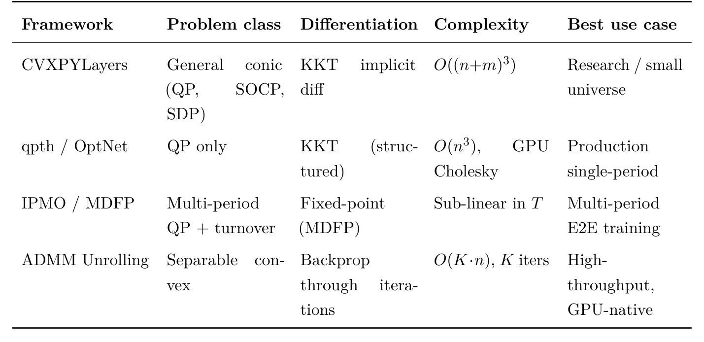
(1) CVXPYLayers — General Conic Programs. CVXPYLayers [18] wraps any convex program expressible in CVXPY (quadratic, second-order cone, semidefinite) as a differentiable PyTorch/JAX layer. Gradients are computed via implicit differentiation through the KKT optimality conditions: given the primal-dual solution (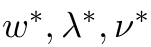), the Jacobian 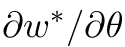is obtained by differentiating the KKT system 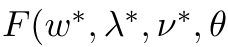) = 0 with respect to parameters θ. This requires solving a linear system of size )) where n is the number of assets and m is the number of constraints—a factorization that scales as 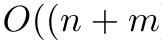)³) in the worst case. Implementation difficulty: Moderate. CVXPYLayers is the most accessible entry point—the convex program is written in declarative CVXPY syntax, and the differentiable wrapper handles KKT differentiation automatically. The primary limitation is runtime: for universes of 500 assets or multi-period horizons 5, the cubic KKT cost becomes a training bottleneck. Suitable for research prototypes and small-to-medium universes.

(2) qpth / OptNet — Quadratic Programs. OptNet [18] specializes to quadratic programs (QPs) of the form min_w ½ 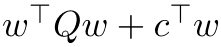 subject to . By restricting to the QP class, the KKT system has a fixed block structure that can be solved more efficiently than the general conic case. Gradients are obtained via the same KKT implicit differentiation, but the structured KKT matrix enables batched GPU-accelerated solves using Cholesky factorization. Implementation difficulty: Low-to-moderate. qpth/OptNet is well-suited to mean-variance optimization where the objective is quadratic in w and constraints are linear. The restriction to QPs is rarely limiting in practice—most portfolio constraints (long-only, leverage, turnover, factor neutrality) are linear. The main limitation is that non-quadratic objectives (CVaR, risk parity) require convex reformulations or approximations. Mature libraries with GPU support make this the preferred choice for production QP layers.

(3) IPMO with MDFP — Multi-Period, Scale-Insensitive. The Integrated Prediction and Multi-period Portfolio Optimization (IPMO) framework [18] addresses the critical limitation of KKT-based methods for multi-period problems. A multi-period optimizer plans a sequence of allocations 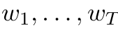jointly, incorporating intertemporal turnover penalties and multi-step transaction costs. Naive KKT differentiation through this program scales as 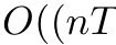)³)— prohibitive for even moderate horizons.

IPMO introduces the Mirror-Descent Fixed-Point (MDFP) differentiation scheme. Rather than factorizing the full KKT system, MDFP computes implicit gradients by iterating a fixed-point equation derived from the mirror-descent optimality conditions. The key property is near horizon-insensitive runtime: as T grows, the per-iteration cost of MDFP grows only weakly (sub-linearly in practice), making multi-period end-to-end training tractable. The mathematical foundation is that the mirror-descent fixed-point = prox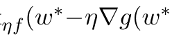)) can be differentiated implicitly without forming the (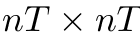) KKT matrix.

Implementation difficulty: High. MDFP requires custom implementation of the fixed-point iteration and its implicit differentiation—no off-the-shelf library wrapper exists as of 2025. The practitioner must implement the mirror-descent updates, convergence checks, and Jacobian-vector products manually. The payoff is substantial: IPMO is the only framework that makes multi-period end-to-end training computationally feasible at scale, and it produces measurably better portfolios by internalizing multi-step transaction costs during training.

(4) ADMM Unrolling — GPU-Parallelisable Iterations. ADMM (Alternating Direction Method of Multipliers) unrolling [18] replaces the convex solver with a fixed number of unrolled ADMM iterations, each of which is a differentiable computation graph node. ADMM splits the optimization into sub-problems that can be solved in closed form (e.g., soft-thresholding for penalties, projection onto the simplex for long-only constraints), making each iteration cheap and GPU-parallelisable across the batch dimension.

The unrolled computation graph has a fixed depth (number of ADMM iterations), and gradients flow through all iterations via standard backpropagation—no implicit differentiation is required. The trade-off is that a fixed iteration count may not achieve convergence for all problem instances, introducing a truncation bias in the gradient estimates. In practice, 20–50 ADMM iterations are sufficient for well-conditioned portfolio problems.

Implementation difficulty: Moderate-to-high. ADMM unrolling requires deriving the ADMM updates for the specific problem structure (the update equations depend on the constraint set and objective), implementing them as differentiable PyTorch operations, and tuning the step size ρ and iteration count. The advantage is that the resulting layer is fully GPU-native and scales well with batch size—making it attractive for high-frequency retraining cycles where throughput matters.

Comparative Summary.

10.2.3 YAND: Matrix-Free Higher-Moment Optimization

The four frameworks above share a common restriction: they optimise mean-variance (quadratic) objectives. All portfolio constraints are linear, and the differentiable Jacobian 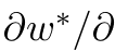ˆµ is derived from a KKT system whose size is 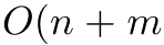). A fifth, qualitatively different class of optimizer has recently been proposed that breaks both assumptions: Yau’s Affine-Normal Descent (YAND), inspired by the paper “Yau’s Affine-Normal Descent for Large-Scale Unrestricted Higher-Moment Portfolio Optimization”, which introduced this framework for large-scale unrestricted higher-moment portfolio optimization. YAND extends the optimizer layer taxonomy to the full mean-variance-skewness-kurtosis (MVSK) objective at institutional universe sizes, while raising new and fundamental questions about end-to-end differentiability.

Algorithm and Geometric Intuition. YAND is a Newton-style descent method whose search direction is defined by the affine normal of the current objective level set rather than the Euclidean gradient or standard Newton step. This geometric choice makes the method invariant to anisotropic affine reparameterizations of the decision space—a property that is particularly valuable for MVSK problems, where the four preference coefficients (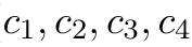) induce strongly anisotropic curvature. At each iterate , YAND assembles the step from: (i) the reduced tangent-space gradient 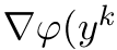), (ii) the tangent Hessian block 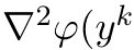), (iii) an affine-normal correction term, and (iv) a single reduced linear solve. The MVSK objective optimised is:

where 0 encode investor preferences for mean return, variance, skewness, and kurtosis respectively. The term unrestricted refers to the absence of factor restrictions or parametric return families—the model works directly from sample moments, which is both empirically appealing and computationally demanding.

Addressing the Curse of Dimensionality.

The central computational barrier to higher-moment portfolio optimization is not statistical but geometric: explicit tensor representations of coskewness and cokurtosis scale as ) and ) in storage, making them practically impossible for universes beyond 50 assets.

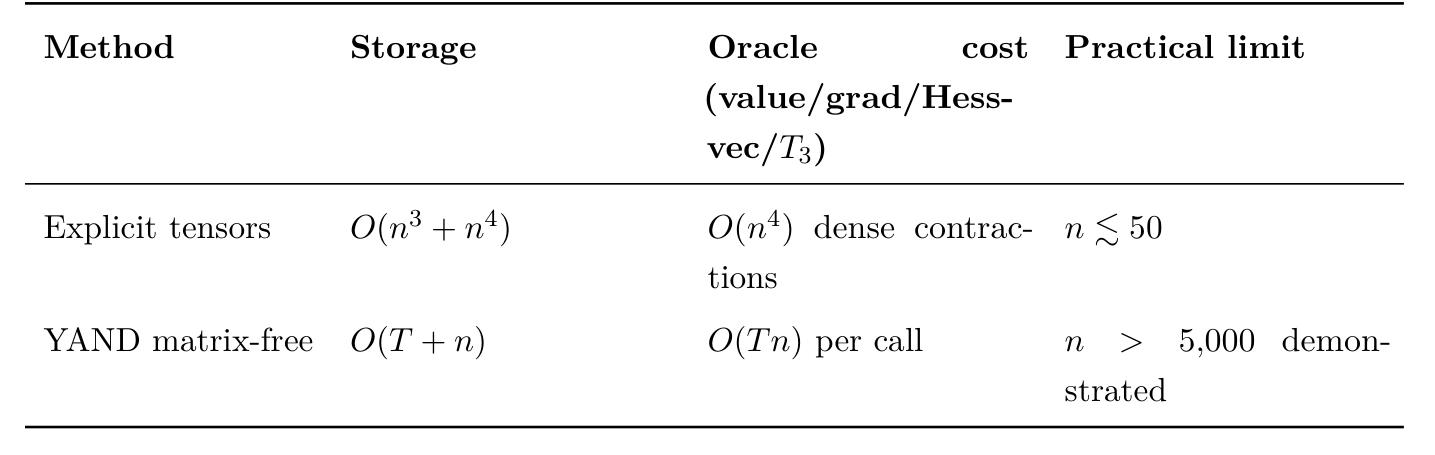
YAND’s key insight is that the MVSK objective and all its derivatives can be expressed entirely through the centered return matrix 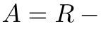1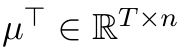 and the projected portfolio return vector :

where denotes elementwise (Hadamard) operations. The gradient, Hessian-vector product 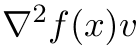, and directional third-order action 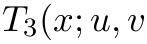) all follow by chain rule from , each requiring only 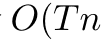) arithmetic and 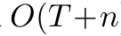) working memory. This is the same asymptotic cost as evaluating a mean-variance objective—YAND achieves ) per oracle call versus ) storage for explicit tensor methods. The method was demonstrated on a cleaned RESSET 5-minute A-share panel with 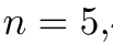440 stocks and T = 66,412 time periods—a problem entirely out of reach for any explicit-tensor higher-moment optimizer.

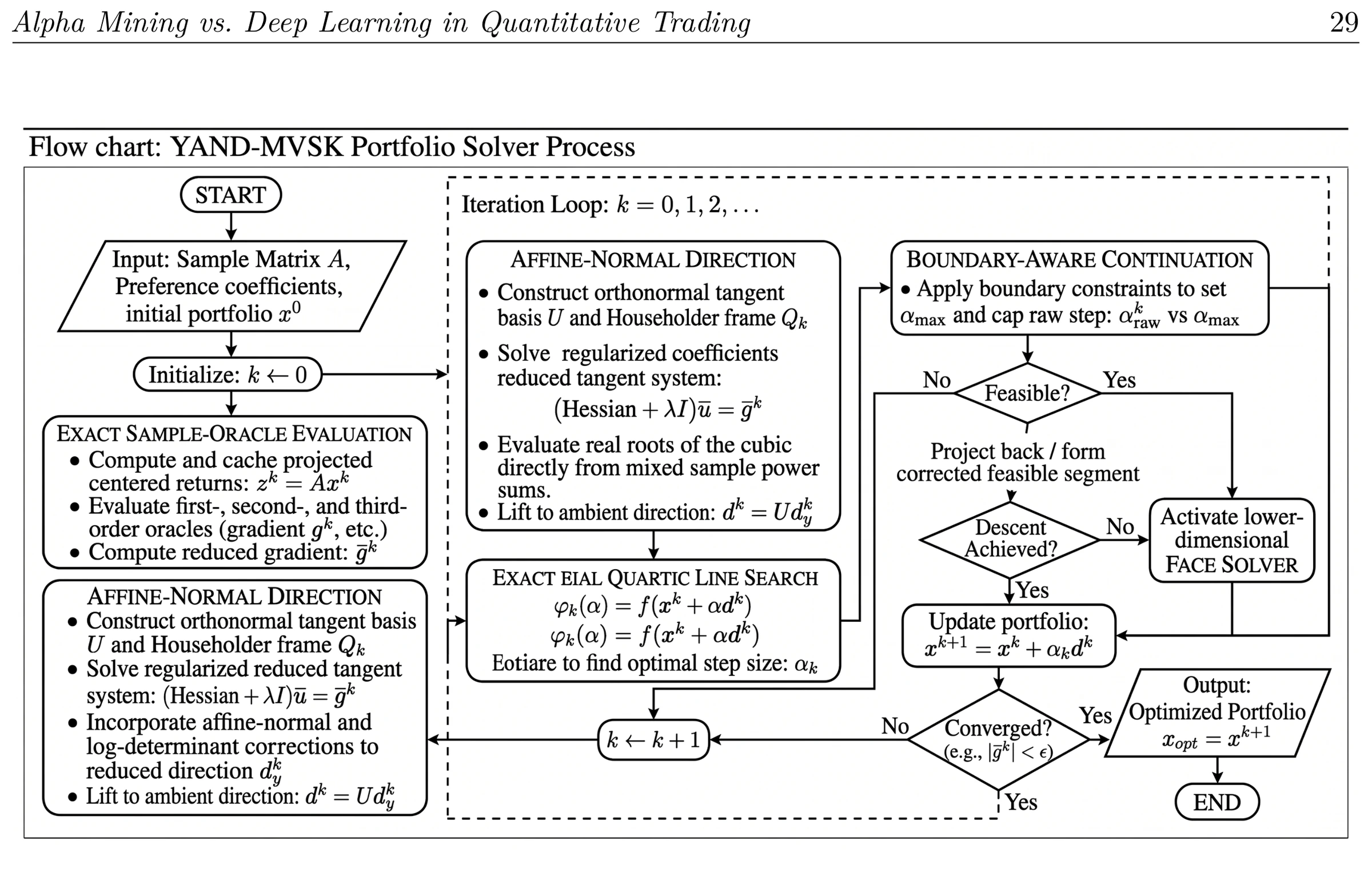
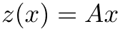
Figure 3 — YAND algorithm flow. Inputs (return matrix R, sample mean µ, preference coefficients c) are combined into the centered return matrix A. All oracle computations (objective, gradient, Hessian-vector, third-order directional action) are performed matrix-free at O(Tn) cost via the projected return vector z(x) = Ax. The affine-normal step is assembled in reduced coordinates on the simplex tangent space, followed by boundary-aware continuation. The algorithm iterates until the tangent-gradient residual ∥∇T f(xk)∥2 ≤ ε. Bottom panels summarize the complexity advantage over explicit-tensor methods and the three structural reasons YAND cannot currently serve as a differentiable E2E layer.

Empirical Results on A-Share Equities. On the real-data panel, MVSK optimization via YAND substantially outperforms mean-variance at moderate return targets. At a 40% annualized return floor (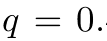40), YAND-MVSK raises the annualized return from 36.24% to 41.68%, the Sharpe ratio from 1.332 to 1.619, while simultaneously improving 1% CVaR and reducing maximum drawdown. The advantage is strongest at moderate return targets, where sufficient design freedom exists to reshape tail exposure; at aggressive targets (60), both MV and MVSK converge to concentrated corner portfolios. These results are particularly relevant to the A-share case study in Section 9: the same high-turnover, retail-dominated market where DL has demonstrated structural advantages also appears to reward kurtosis-aware allocation, suggesting complementary rather than competing improvements.

End-to-End Optimization Compatibility. The critical question for DL system design is whether YAND can serve as a differentiable optimizer layer—i.e., whether gradients of the portfolio performance loss can flow through YAND back into the prediction network. This

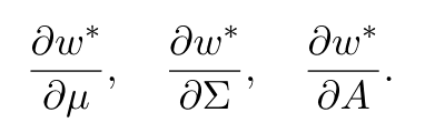
There are three structural reasons why YAND cannot currently serve as a differentiable E2E layer:

1. (1) No implicit differentiation derivation. The paper derives oracle computations for , , and 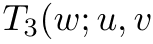)—all derivatives with respect to the decision variable w. It does not derive or discuss 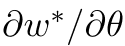for any input parameter θ. The KKT conditions for the MVSK problem involve third-order terms, and differentiating through them to obtain 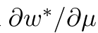would require solving a linear system involving —non-trivial even in the matrix-free setting.
2. (2) Variable-depth Newton architecture, not unrollable. Unlike ADMM unrolling (fixed number of iterations forming a static computation graph) or MDFP (fixed-point equation enabling implicit differentiation), YAND is a variable-depth Newton method: it runs until convergence, with the number of iterations depending on the problem instance. This variable depth makes unrolling impractical—one cannot differentiate through an unknown number of steps in a standard autograd framework.
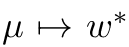
3. (3) Boundary-aware continuation is non-smooth. YAND’s simplex feasibility mechanism involves conditional branching: if a trial step violates the simplex boundary, the algorithm projects back and activates a lower-dimensional face solver. These branching decisions are nondifferentiable—the computational graph has discrete forks that break backpropagation. While the reduced-coordinate oracle computations are individually differentiable (confirmed via chain rule), the overall input-output map is not smooth at boundary-active solutions. Theoretical Path to Differentiability. Differentiability is not impossible in principle—it is simply absent from the current paper. For interior solutions where 0 component-wise (no binding long-only constraints), the KKT conditions reduce to 1. Differentiating implicitly with respect to µ:

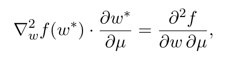
a linear system solvable with one Hessian-vector product at the same ) cost as a YAND oracle call. A future YAND-Layer could implement this for interior solutions, analogous to how CVXPYLayers implements KKT implicit differentiation for convex programs. This would require:

1. (a) deriving the cross-partial 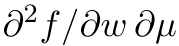in the matrix-free setting, (b) handling boundary cases where the implicit function theorem fails, and (c) wrapping the result in an autograd-compatible interface. None of this exists today, but the theoretical machinery is present in the paper’s oracle framework. Comparison: YAND vs. End-to-End Optimization. Because YAND operates in a two-stage paradigm (predict µ separately, then optimize), the comparison with E2E systems is not about optimizer quality in isolation, but about what the two-stage versus joint-training gap costs, and whether YAND’s higher-moment capability compensates.

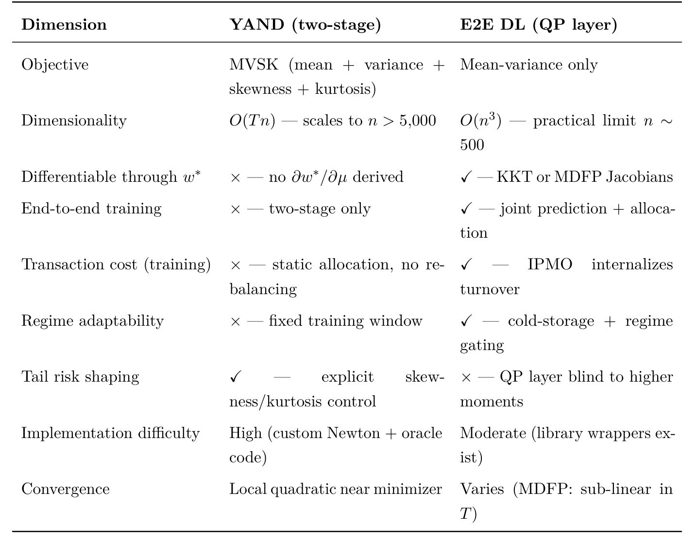
YAND has a structural advantage wherever tail-risk shaping is the primary objective: the A-share evidence shows a Sharpe improvement of +22% over mean-variance at moderate return targets, a dimension of portfolio quality that current E2E DL optimizer layers are structurally blind to. E2E systems retain their advantage in joint prediction-allocation alignment, transaction cost internalization during training, and dynamic regime adaptability—all of which are absent from YAND’s static allocation design.

The Hybrid Possibility. The most practically interesting implication is a staged hybrid: a DL prediction network (E2E trained with a QP layer for mean-variance) feeds its return forecasts ˆµ into YAND as the terminal allocation step at inference time. This would: (i) preserve E2E training’s alignment of prediction with portfolio performance via the QP layer during training; (ii) apply YAND’s higher-moment reshaping at inference using the E2E-trained ˆµ; and (iii) benefit from YAND’s scalability to large universes at the allocation stage. The cost is a train-test mismatch: the prediction model was aligned to a QP optimizer during training, but at inference it feeds a YAND-MVSK optimizer. Whether this misalignment is tolerable in practice is an open empirical question, but the magnitude of YAND’s higher-moment gains suggests that even an imperfectly aligned predictor may benefit substantially from kurtosis-aware allocation. This hybrid design represents a promising direction for future research at the intersection of differentiable optimization and higher-moment portfolio theory.

10.2.4 End-to-End Training and Gradient Flow

The defining advantage of a differentiable optimizer layer over a classical two-stage pipeline is that gradients of the portfolio performance loss flow through the optimizer and back into the prediction network. In a two-stage system, the prediction model is trained to minimize forecast error (e.g., mean squared error on returns), and the optimizer is applied post-hoc. This decoupling means the prediction model is not aware of how its forecasts will be used—a misalignment that can produce high-accuracy forecasts that translate to poor portfolio performance due to transaction costs, risk constraints, or factor exposures.

In an end-to-end system, the training objective is directly a portfolio performance metric— realized Sharpe ratio, net-of-cost return, or a distributionally robust portfolio objective. The gradient of this objective with respect to the prediction network’s parameters θ is:

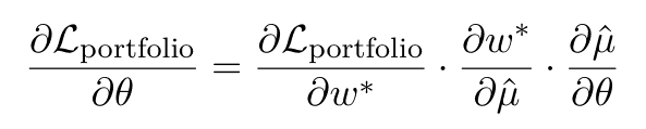
where 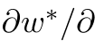ˆµ is the Jacobian of the optimizer’s solution with respect to its return input—the quantity computed by the differentiable solver. This Jacobian encodes how the optimizer uses the prediction: assets with high sensitivity ˆ are those for which better predictions most directly improve portfolio performance, focusing the prediction network’s learning capacity where it matters most.

10.2.5 Residual Factor Hedging

A specialized component of the portfolio optimizer layer is the residual factor hedging module, which generates hedging signals to remove common market exposures from the portfolio. This module addresses the factor crowding problem directly: by predicting the residual returns after removing common factor exposures, the DL system can generate signals that are orthogonal to the crowded factor space, providing diversification that alpha mining approaches struggle to achieve [18].

10.3 Adaptive and Dynamic Trading Mechanism Layers

Beyond the portfolio optimizer, a full DL trading system includes several adaptive trading mechanism layers that dynamically adjust the system’s behavior in response to changing market conditions:

10.3.1 Dynamic Signal Weighting

Rather than using fixed weights to combine predictions from multiple model snapshots, an adaptive weighting layer learns to assign weights based on current market conditions. This is implemented as a meta-model that takes current market state as input and outputs a weight vector over the cold-storage library, effectively selecting the most relevant historical model for current conditions.

10.3.2 Regime Gating and Modular Routing

Regime-aware architectures (RegimeNAS) route the input feature matrix through different specialized sub-networks depending on the detected market regime. The regime detection itself is learned from data, not pre-specified, allowing the system to identify regime boundaries that are not obvious to human observers [6]. The specialized sub-networks (volatility block, trend block, range block) are each optimized for their respective regime types, producing predictions that are more accurate within each regime than a single general-purpose model.

10.3.3 Online Adaptation Layers

For high-frequency strategies, the latency of full model retraining is prohibitive. Online adaptation layers—implemented as lightweight parameter updates applied to the model’s final layers—allow the system to adapt to very recent market dynamics without full retraining. These layers can be updated on a daily or intraday basis, providing a form of continuous learning that bridges the gap between the model’s training distribution and current market conditions.

10.3.4 Execution Intelligence Layer

The execution intelligence layer translates the portfolio optimizer’s target weights into actual orders, accounting for market microstructure dynamics (bid-ask spread, market impact, queue position) in real time. This layer is implemented as a separate DL model trained on historical execution data, and its quality is a significant source of alpha leakage prevention—a capability that is largely absent in alpha mining pipelines, which typically use simple execution algorithms.

10.4 Overfitting and Alpha-Decay Mitigation Systems

Well-engineered DL systems implement a multi-layer defense against overfitting and alpha decay:

10.4.1 Architectural Regularization

• Lipschitz stability constraints: Lipschitz bounds on the model’s weight matrices constrain the sensitivity of predictions to input perturbations, reducing overfitting to noise in the training data [6];
• Dropout and variational inference: standard dropout regularization is augmented with variational inference techniques that produce calibrated uncertainty estimates, enabling the system to distinguish between high-confidence and low-confidence predictions;
• Depth and width control: architecture search (NAS) is used to find the minimumcomplexity model that achieves the required predictive performance, avoiding the overpa-rameterization that is the primary driver of overfitting in large neural networks.

10.4.2 Label Engineering

• Triple-barrier labeling: rather than using raw returns as training labels, the triplebarrier method labels observations based on which of three barriers (profit target, stop-loss, or time limit) is hit first, producing labels that are more robust to noise and more aligned with actual trading objectives [19];
• Noise augmentation: controlled noise is added to training inputs to improve the model’s robustness to measurement error and data quality issues;
• Amplitude and time-scale invariance: inductive biases that enforce invariance to scaling and temporal shifts in the input features, improving generalization to nonstationary markets [7].

10.4.3 Backtest Overfitting Detection

A dedicated overfitting detection layer screens candidate models before deployment using hypothesis testing frameworks that estimate the probability that a model’s backtest performance is attributable to genuine predictive skill rather than curve-fitting. Models that fail this screen are returned to the cold-storage library without being deployed, preventing the accumulation of overfitted strategies in the production system.

10.4.4 Half-Life Monitoring and Decay Detection

Each deployed model snapshot is monitored for alpha decay using half-life diagnostics: the model’s live Sharpe ratio is tracked against a decay curve calibrated on historical performance, and models whose live performance falls below the expected decay curve are automatically downweighted or retired. This monitoring system is analogous to the signal-level decay monitoring in alpha mining, but operates at the model level rather than the signal level.

10.5 Regime-Aware Architecture Compounding

The final source of compounding moat is regime-aware architecture compounding: the process by which the system’s architecture search capabilities improve over time as the cold-storage library grows. When the cold-storage library contains model snapshots from many historical regimes, the architecture search process can use this library as a training set for meta-learning: learning to quickly adapt to new regimes by drawing on the experience of adapting to historical regimes. This is the quantitative analogue of the human expert’s ability to recognize a new market regime as “similar to 2008” or “similar to the 2020 COVID crash” and apply appropriate strategies. As the library grows, the meta-learning capability improves, and the system becomes progressively better at adapting to new regimes—a compounding advantage that has no direct analogue in alpha mining, where each new regime is addressed by mining new signals from scratch.

11 System and Pipeline Architecture

11.1 Alpha Mining Pipeline

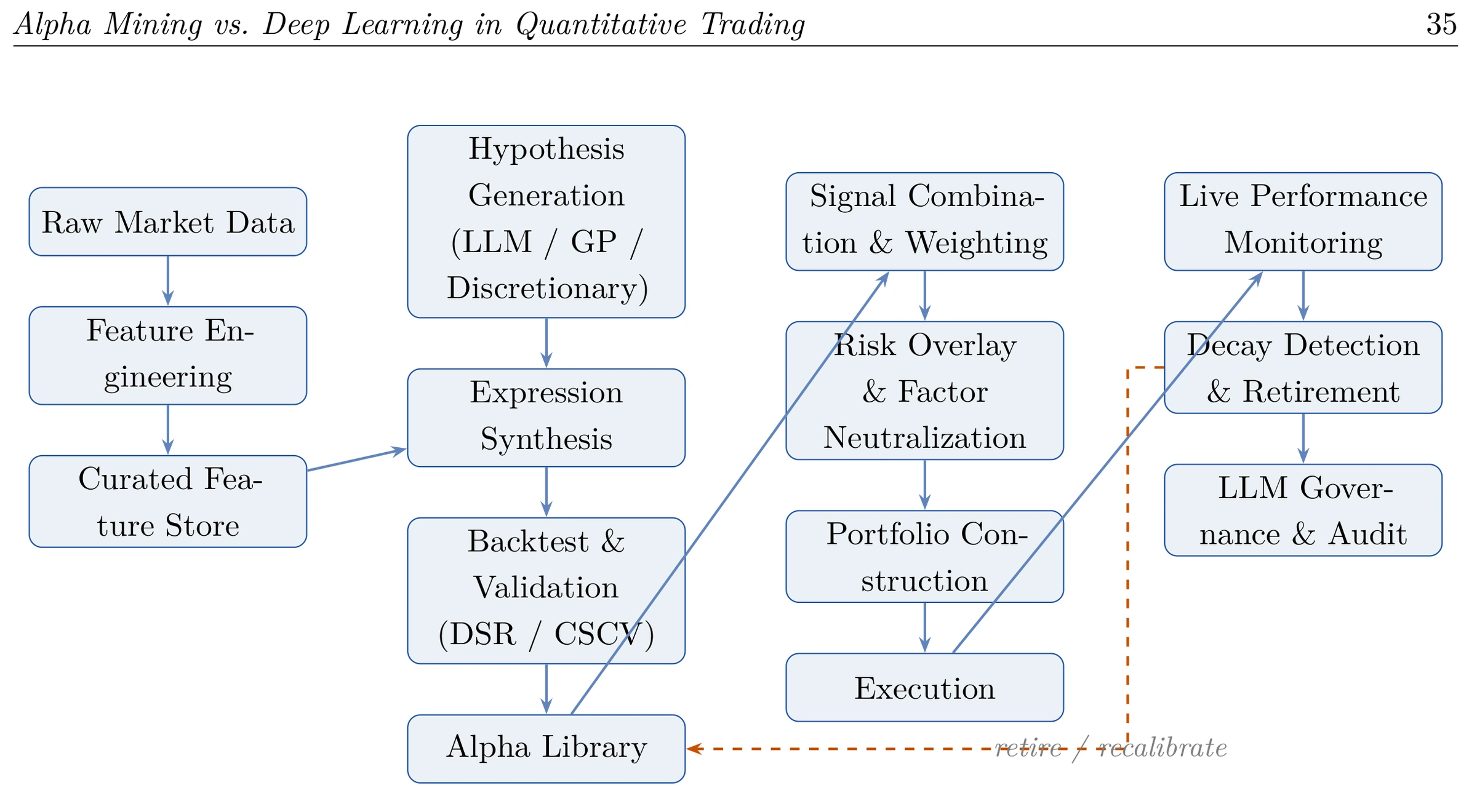
Figure 4 — describes the alpha mining pipeline architecture.

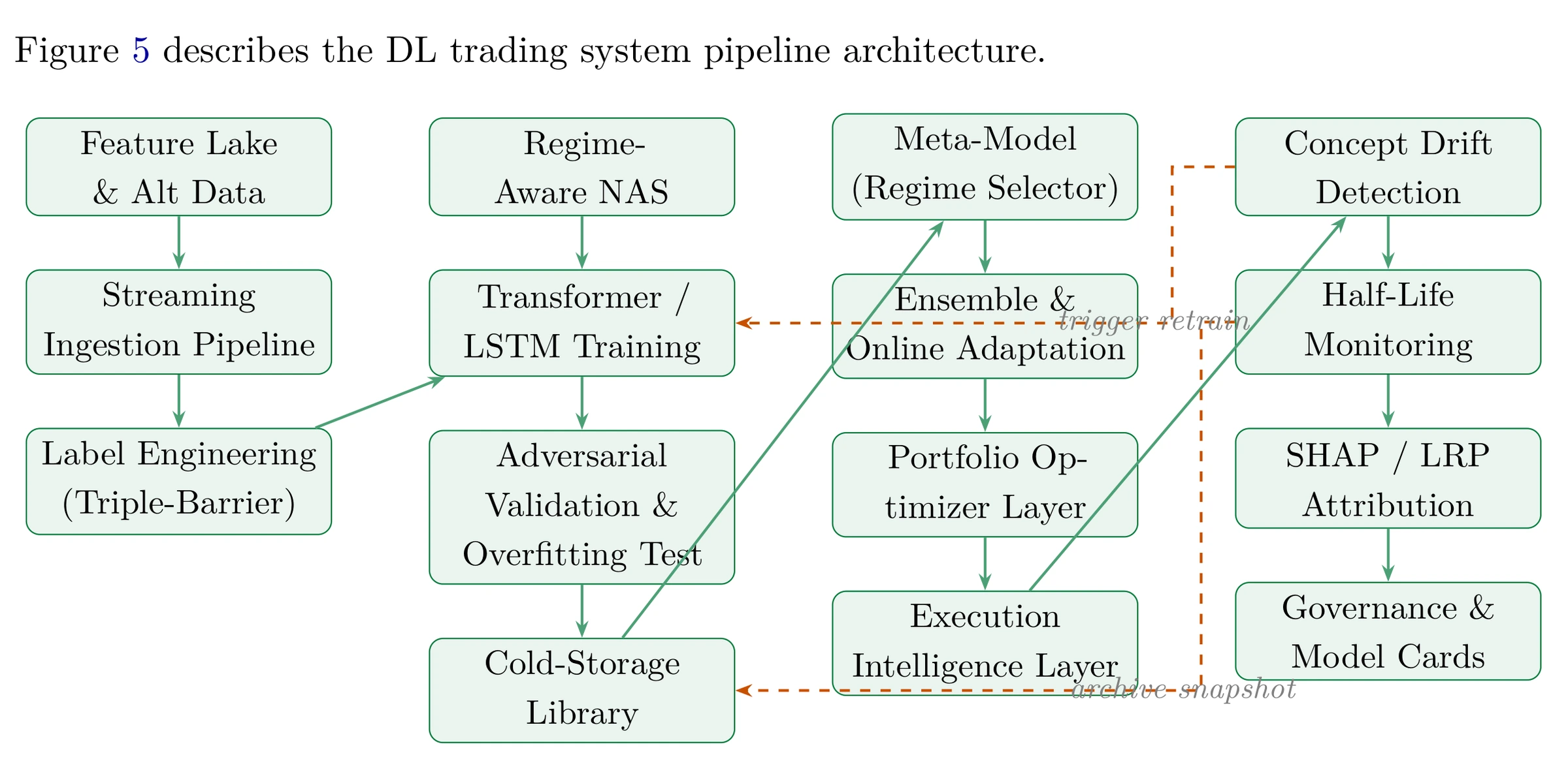
Raw Market Data (LLM / GP / Discretionary) Feature Engineering Expression Synthesis Curated Feature Store Backtest & Validation (DSR / CSCV) Alpha Library Feature Lake Regime-& Alt Data Aware NAS Streaming Transformer / Ingestion Pipeline LSTM Training Label Engineering Adversarial (Triple-Barrier) Validation & Overfitting Test Cold-Storage Library

11.3 Comparative Pipeline Analysis

Signal Combina-Live Performance tion & Weighting Monitoring Risk Overlay Decay Detection & Factor & Retirement Neutralization LLM Gover-Portfolio Con-nance & Audit struction Execution retire / recalibrate Meta-Model Concept Drift (Regime Selector) Detection Half-Life Ensemble & trigger retrain Monitoring Online Adaptation SHAP / LRP Portfolio OpAttribution timizer Layer Governance & Execution Model Cards Intelligence Layer archive snapshot

11.2 Deep Learning Trading System Pipeline

Figure 5 — describes the DL trading system pipeline architecture.

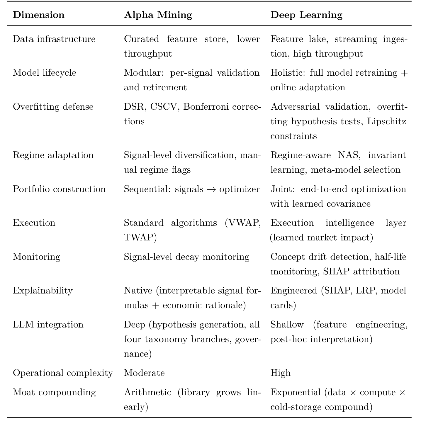
12 A Framework for Paradigm Selection

Given the multidimensional analysis above, we propose a Paradigm Selection Framework based on four organizational and market-structure dimensions:

12.1 Organizational Capability Assessment

(1) Compute access: Does the organization have sustained access to GPU clusters sufficient for periodic model retraining? If not, alpha mining is the appropriate primary paradigm. (2) Data breadth: Does the organization have access to large, diverse, high-quality datasets including alternative data? If not, DL’s expressive power is constrained and alpha mining is more efficient.

1. (3) ML engineering depth: Does the organization have dedicated ML engineers capable of building and maintaining the DL pipeline components described in Section 11? If not, the operational complexity of DL is prohibitive.
2. (4) Regulatory environment: Is the organization subject to strict explainability requirements? If so, alpha mining’s native interpretability (across all four taxonomy branches) is a significant advantage.

12.2 Market-Structure Assessment

1. (1) Retail participation: What fraction of daily volume is retail? Higher retail participation favors DL.
2. (2) Nonlinearity: Are price dynamics dominated by nonlinear, behavioral, and sentimentdriven patterns? Higher nonlinearity favors DL.
3. (3) Fundamental anchor: Is there a stable fundamental valuation framework? Stronger fundamental anchors favor alpha mining.
4. (4) Factor crowding: Are linear factor premia already crowded? Higher crowding favors DL’s ability to discover non-crowded, proprietary representations.

12.3 Recommended Paradigm Choices

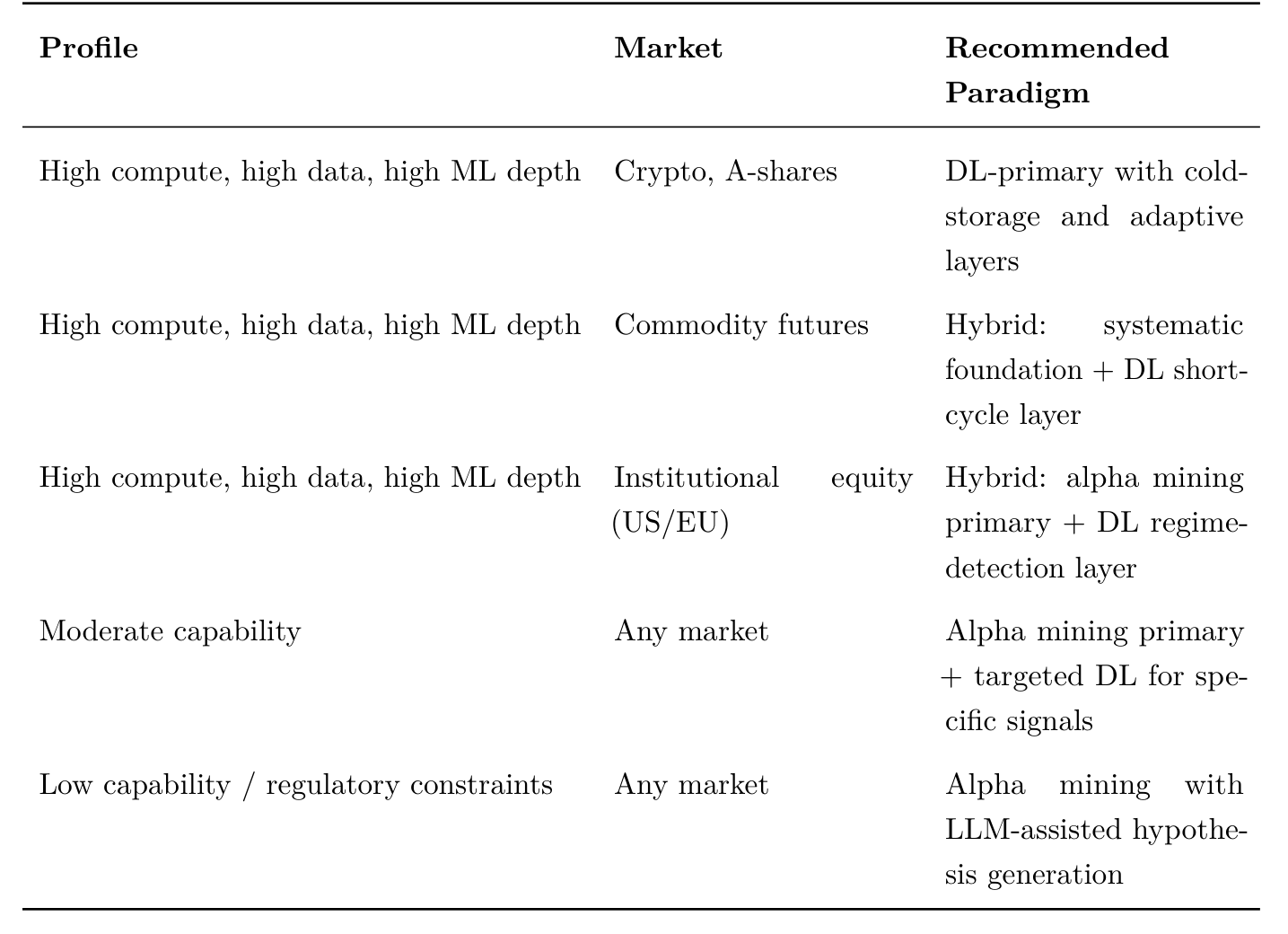
12.4 The Hybrid Architecture as a Plausible Option

The foregoing analysis suggests that hybrid architectures—combining systematic alpha mining and deep learning components—represent a plausible and attractive option for well-resourced quantitative funds, though not the inevitable long-run equilibrium. Whether a hybrid is optimal depends critically on organizational capability, target market, and investment horizon. For firms with deep DL expertise and sustained compute access operating in behavioral markets, a DL-primary architecture may be superior. For firms with strong discretionary research culture operating in institutionally dominated markets, a systematic-primary architecture may be more efficient. The hybrid is best understood as a risk-managed transition architecture or a diversification strategy rather than a universal optimum.

12.5 Detailed Hybrid System Design

For organizations that do elect to pursue a hybrid architecture, Figure 6 presents a detailed system design that integrates both paradigms into a coherent, production-grade pipeline.

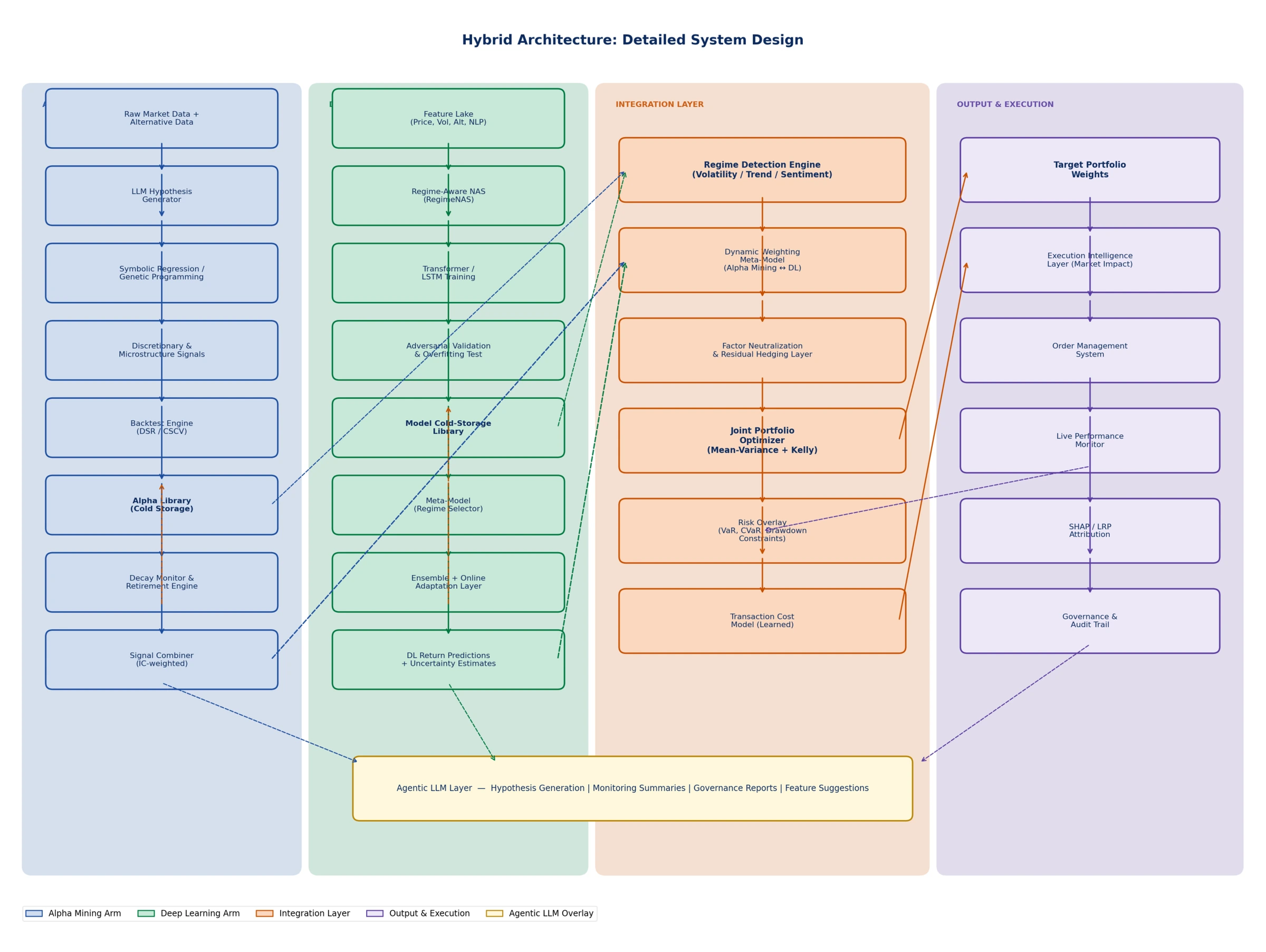
Figure 6 — Detailed hybrid architecture system design. Four functional lanes—Alpha Mining Arm, Deep Learning Arm, Integration Layer, and Output & Execution—are orchestrated by a Regime Detection Engine and integrated through a joint portfolio optimizer. An Agentic LLM overlay provides hypothesis generation, monitoring summaries, and governance support across all lanes.

The hybrid system design comprises four functional lanes:

12.5.1 Alpha Mining Arm

The alpha mining arm operates as a self-contained research and production pipeline:

• LLM Hypothesis Generator: an agentic LLM layer that continuously generates, ranks, and operationalizes candidate signal hypotheses from all four branches of the broadened taxonomy (Section 2);
• Symbolic Regression / Genetic Programming Engine: automated search over operator trees, constrained by originality checks (AST similarity) and complexity caps to prevent crowded or overfitted signals;
• Discretionary & Microstructure Signals: a curated set of signals derived from domain expertise, order flow analysis, and bid-ask dynamics, maintained by human researchers;
• Backtest Engine (DSR/CSCV): rigorous out-of-sample validation with deflated Sharpe ratio and combinatorially symmetric cross-validation to screen for overfitting;
• Alpha Library (Cold Storage): a versioned repository of validated signals with full metadata (Sharpe, decay half-life, correlation profile, regime sensitivity, discovery date);
• Decay Monitor & Retirement Engine: continuous monitoring of live signal performance against expected decay curves; automatic downweighting and retirement of decaying signals;
• Signal Combiner (IC-weighted): combination of active signals using information coefficient (IC)-weighted averaging, with correlation constraints to maintain diversification.

12.5.2 Deep Learning Arm

The deep learning arm operates as a parallel, model-centric pipeline:

• Feature Lake: a high-throughput data store ingesting price, volume, fundamental, alternative, and NLP features across all instruments and time horizons;
• Regime-Aware NAS (RegimeNAS): differentiable architecture search that jointly optimizes model architecture and regime-specific routing, producing architectures with Lipschitz stability guarantees;
• Transformer / LSTM Training: end-to-end model training with triple-barrier labeling, noise augmentation, and variational output heads for uncertainty estimation;
• Adversarial Validation & Overfitting Test: hypothesis-testing framework that screens candidate models for backtest overfitting before admission to the cold-storage library;
• Model Cold-Storage Library: versioned repository of trained model snapshots, each tagged with training period, market regime characteristics, and performance metrics;
• Meta-Model (Regime Selector): a lightweight model that queries the cold-storage library and selects the most regime-appropriate snapshot(s) for current market conditions;
• Ensemble + Online Adaptation Layer: ensemble combination of selected snapshots with online parameter updates applied to final layers for rapid adaptation to recent market dynamics;
• DL Return Predictions + Uncertainty Estimates: distributional output combining point predictions with calibrated uncertainty estimates for downstream risk sizing.

12.5.3 Integration Layer

The integration layer is the architectural core of the hybrid system, responsible for combining the outputs of both arms and translating them into a coherent portfolio:

• Regime Detection Engine: a dedicated model that continuously classifies the current market regime across multiple dimensions (volatility level, trend strength, sentiment state, liquidity condition). This engine drives the dynamic weighting of the two arms;
• Dynamic Weighting Meta-Model: given the current regime classification, this model outputs a weight vector (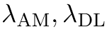) that determines the relative contribution of the alpha mining and DL arms to the combined signal. In trending, institutionally dominated regimes, is higher; in behavioral, high-volatility regimes, is higher;
• Factor Neutralization & Residual Hedging Layer: the combined signal is projected onto the null space of common factor exposures, removing crowded factor tilts and producing a factor-neutral alpha signal;
• Joint Portfolio Optimizer: solves the mean-variance optimization problem with the combined, factor-neutral signal as input, incorporating learned covariance estimates, Kelly-fractional position sizing for high-confidence predictions, and hard constraints on leverage, turnover, and concentration;
• Risk Overlay: enforces real-time VaR, CVaR, and drawdown constraints, with dynamic position scaling during stress periods;
• Transaction Cost Model (Learned): a DL model trained on historical execution data that predicts market impact and adjusts the optimization objective to account for trading costs.

12.5.4 Output & Execution

• Target Portfolio Weights: the final output of the optimization pipeline, expressed as a vector of instrument weights;
• Execution Intelligence Layer: a learned model of optimal order scheduling that minimizes market impact by adapting to intraday liquidity patterns;
• Order Management System: routes orders to appropriate venues with pre-trade risk checks;
• Live Performance Monitor: tracks realized performance against expectations for both arms and all individual signals/models;
• SHAP / LRP Attribution: generates post-hoc explanations of portfolio decisions for governance review and regulatory compliance;
• Governance & Audit Trail: maintains a complete, reproducible record of all decisions, model versions, and data inputs.

12.5.5 Agentic LLM Overlay

A crosscutting agentic LLM layer provides services to all four functional lanes:

• To the Alpha Mining Arm: hypothesis generation, signal documentation, crowding detection, and literature monitoring;
• To the Deep Learning Arm: feature engineering suggestions, architecture search guidance, and post-hoc interpretation synthesis;
• To the Output & Execution lane: natural-language monitoring summaries, anomaly explanations, and governance report generation.

13 Conclusion

This paper has provided a comprehensive, multidimensional comparison of systematic alpha mining and deep learning approaches to quantitative alpha generation. The central findings are:

1. (1) Neither paradigm is universally superior. The relative advantage of each is determined by market microstructure, organizational capability, and investment horizon. The Market-Structure Principle provides a principled basis for paradigm selection.
2. (2) Deep learning’s advantage is structural in behavioral markets. In markets dominated by retail participation, nonlinear dynamics, and absent fundamental anchors (cryptocurrency, Chinese A-shares, short-cycle commodity futures), DL architectures are structurally better suited to capturing the dominant predictive patterns. This is not a claim about model quality but about the alignment between model architecture and market dynamics.
3. (3) Well-engineered DL systems compound their moat. The compounding moat argument is the paper’s most original contribution. Through cold-storage libraries, regime-aware architecture search, adaptive trading mechanism layers, and end-to-end portfolio optimization, DL systems accumulate institutional memory and pipeline depth that grow with every market cycle. This compounding dynamic has no direct analogue in alpha mining, where the moat is primarily a function of library size and process quality.
4. (4) Agentic LLMs are a force multiplier for alpha mining. The natural language interface of agentic LLMs aligns closely with the hypothesis-driven, iterative nature of systematic alpha discovery. For DL systems, LLMs play a useful but peripheral role.
5. (5) Hybrid architectures are the long-run equilibrium. The optimal system combines systematic and DL components, with a regime-aware meta-model dynamically weighting their contributions. The specific mix depends on organizational capability and target market.
6. (6) Intellectual honesty requires acknowledging evidence quality. Much of the evidence cited in this paper derives from academic backtests and preprints rather than verified live performance data. The structural arguments are supported by theory and empirical patterns, but practitioners should apply appropriate skepticism to specific performance claims. The quantitative trading landscape in 2026 is one in which the tools for both paradigms are maturing rapidly, the competitive field is intensifying, and the alpha half-life across all approaches is shortening. In this environment, the most defensible position is not a bet on either paradigm but an investment in the organizational capability to execute both—and to compound the moat that each generates through disciplined, systematic engineering.

References

[1] WorldQuant. (2023). Alpha research and systematic signal discovery: A practitioner’s perspective. Working paper.

[2] Wang, Y., Li, Y., & Liu, X. (2024). Alpha-GPT: Human-AI interactive alpha mining for quantitative investment. arXiv preprint arXiv:2308.00016. doi:10.48550/arXiv.2308.00016

[3] Ma, T., Wang, W., & Chen, Y. (2023). Attention is all you need: An interpretable transformer-based asset allocation approach. International Review of Financial Analysis, 88, 102876. doi:10.1016/j.irfa.2023.102876

[4] Bailey, D. H., & López de Prado, M. (2014). The deflated Sharpe ratio: Correcting for selection bias, backtest overfitting, and non-normality. Journal of Portfolio Management, 40(5), 94–107. doi:10.3905/jpm.2014.40.5.094

[5] Bailey, D. H., Borwein, J., López de Prado, M., & Zhu, Q. J. (2015). The probability of backtest overfitting. Journal of Computational Finance, 20(4), 39–69. doi:10.21314/JCF.2017.322

[6] Devadiga, P., & Shailesh, Y. (2025). RegimeNAS: Regime-aware differentiable architecture search with theoretical guarantees for financial trading. arXiv preprint arXiv:2508.11338. doi:10.48550/arXiv.2508.11338

[7] Zhang, Z., Chen, B.-C., & Zhu, S. (2024). From attention to profit: Quantitative trading strategy based on transformer. arXiv preprint arXiv:2404.00424. doi:10.48550/arXiv.2404.00424

[8] Lim, B., & Zohren, S. (2021). Time-series forecasting with deep learning: A survey. Philosoph- ical Transactions of the Royal Society A, 379(2194), 20200209. doi:10.1098/rsta.2020.0209

[9] Coletta, A., Vyetrenko, S., & Balch, T. (2023). Towards robust trading strategy design with adversarial training. arXiv preprint arXiv:2302.03690. doi:10.48550/arXiv.2302.03690

[10] Ozbayoglu, A. M., Gudelek, M. U., & Sezer, O. B. (2020). Deep learning for financial applications: A survey. Applied Soft Computing, 93, 106384. doi:10.1016/j.asoc.2020.106384

[11] Cao, L. (2024). Explainable AI for finance: Challenges and prospects. IEEE Intelligent Systems, 39(1), 12–21. doi:10.1109/MIS.2024.3350842

[12] Volpati, V., Benzaquen, M., Eisler, Z., Bouchaud, J.-P., & Bucci, F. (2020). Zooming in on equity factor crowding. SSRN Working Paper. doi:10.2139/SSRN.3518404

[13] Ke, Z. T., Kelly, B. T., & Xiu, D. (2019). Predicting returns with text data. NBER Working Paper No. 26186. doi:10.3386/w26186

[14] Xu, R. (2025). High-dimensional spatiotemporal dependencies and behavioral heterogeneity co-modeling: LSTM-multi-factor penetrative analysis and risk premium decomposition of the reversal effect in China’s A-share market. Proceedings of the ACM International Conference on Computing and Data Science. doi:10.1145/3746972.3746984

[15] Zhang, Z., Chen, B.-C., Zhu, S., et al. (2024). From attention to profit: Quantitative trading strategy based on transformer. arXiv preprint arXiv:2404.00424. doi:10.48550/arXiv.2404.00424

[16] Zhou, F., Zhang, Q., & Zhu, Y. (2022). T2V_TF: An adaptive timing encoding mechanism based transformer with multi-source heterogeneous information fusion for portfolio management. Expert Systems with Applications, 213, 119020. doi:10.1016/j.eswa.2022.119020

[17] Li, B., Xie, K., Lu, S., et al. (2020). LSTM-based quantitative trading using dynamic K-top and Kelly criterion. Proceedings of IJCNN 2020. doi:10.1109/IJCNN48605.2020.9207264

[18] Imajo, K., Minami, K., Ito, K., & Nakagawa, K. (2020). Deep portfolio optimization via distributional prediction of residual factors. arXiv preprint arXiv:2012.07245. doi:10.48550/arXiv.2012.07245

[19] López de Prado, M. (2018). Advances in Financial Machine Learning. John Wiley & Sons.

[20] Huang, S. (2024). Enhancing investment strategies through machine learning: A comprehensive analysis across market sectors. Applied and Computational Engineering, 104. doi:10.54254/2755-2721/104/20240909

[21] Jiang, Z., Xu, D., & Liang, J. (2017). A deep reinforcement learning framework for the financial portfolio management problem. arXiv preprint arXiv:1706.10059. doi:10.48550/arXiv.1706.10059

[22] Bieganowski, B., & Ślepaczuk, R. (2024). Supervised autoencoder MLP for financial time series forecasting. arXiv preprint arXiv:2404.01866. doi:10.48550/arXiv.2404.01866